\(~~~~~~~~~\)Probability and Statistics\(~~~~~~~~~\)
Asst. Prof. Dr. Somsak Chanaim
International College of Digital Innovation, CMU
August 14, 2026
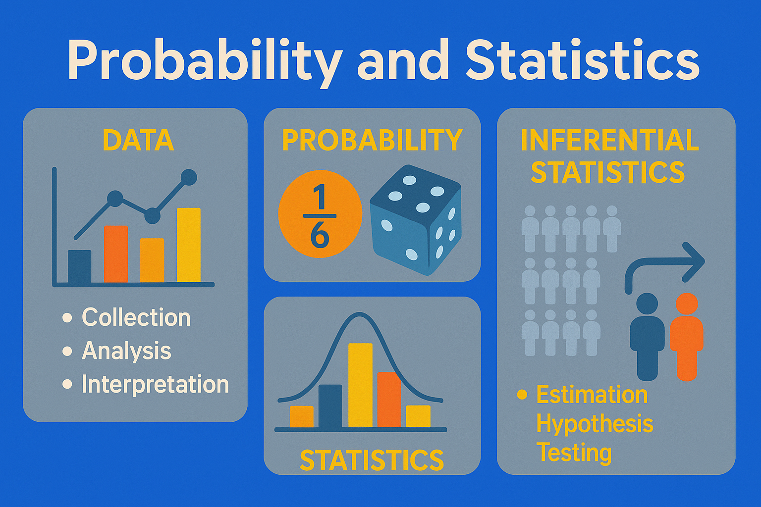
Axiom of Probability
Axioms of Probability are three fundamental rules that define the properties of probability.
They were proposed by Andrey Kolmogorov in 1933 and form the foundation of modern probability theory.

Kolmogorov’s Axioms: Let \(S\) be a sample space and let \(A\) be any event that is a subset of \(S\).
Example 1: Tossing a fair coin

Sample space \(S\):
All possible outcomes \[
S = \{\text{Heads}, \text{Tails}\}
\] Event \(A\): Getting a Head \[
A = \{\text{Heads}\}
\]
Example 2: Rolling a six-sided die
Sample space \(S\): \[ S = \{1, 2, 3, 4, 5, 6\} \] Event \(A\): Rolling an even number \[ A = \{2, 4, 6\} \]

Example 3: Drawing a card from a standard 52-card deck

Sample space \(S\): All 52 unique cards \[ S = \{\text{Ace of Hearts}, \text{2 of Hearts},\\ \ldots, \text{King of Spades}\} \] Event \(A\): Drawing a red card
\[A = \{\text{all Hearts and Diamonds}\\ \text{(26 cards)}\}\]
The three axioms are as follows:
Axiom 1 Probability must be non-negative
\[P(A) \geq 0\]
For every event \(A\), this means the probability must always be a non-negative value—either positive or at least zero.
Axiom 2 The probability of the sample space is 1
\[P(S) = 1\]
This means the probability of the event that covers all possible outcomes must equal 1.
Axiom 3 Additivity for mutually exclusive events
If \(A\) and \(B\) are mutually exclusive events, meaning they have no outcomes in common (i.e., \(A \cap B = \emptyset\)), then
\[
P(A \cup B) = P(A) + P(B)
\]
This means if two events cannot occur at the same time, the probability of either one occurring is the sum of their individual probabilities.
Results Derived from the Axioms of Probability
From the three axioms, we can infer other important properties. For example:
The probability of an impossible event is zero
\[P(\emptyset) = 0\]
An impossible event has a probability of zero because it cannot occur.
Complement Rule
\[P(A^c) = 1 - P(A)\]
This means that if the probability of event \(A\) is \(P(A)\), then the probability of the event not \(A\) is \[1−P(A)1−P(A)\]
General Addition Rule of Probability
For any events \(A\) and \(B\):
\[P(A \cup B) = P(A) + P(B) - P(A \cap B)\]
This formula applies even when the events may overlap.
Example Applying the Axioms of Probability
Rolling a single die
Let \(S = \{1, 2, 3, 4, 5, 6\}\)
- Event \(A\): rolling an odd number → \(A = \{1, 3, 5\}\)
- Event \(B\): rolling a number greater than 4 → \(B = \{5, 6\}\)
- \(P(A) = \frac{3}{6} = 0.5\), \(P(B) = \frac{2}{6} = 0.333\),
\(P(A \cap B) = \frac{1}{6} = 0.167\)
Using the addition rule: \[P(A \cup B) = P(A) + P(B) - P(A \cap B)\]
\[= 0.5 + 0.333 - 0.167 = 0.666\]
🚪 Monty Hall Game
(async () => {
  const uid = "mh_final_v2_" + Math.random().toString(36).substr(2, 9);

  const box = html`<div style="width:100%; display:flex; justify-content:center; font-family:'Sarabun', system-ui, sans-serif; color:#334155;">
    <style>
      .mh-wrapper {
        width: 100%; max-width: 800px;
        background: white; padding: 25px; border-radius: 16px;
        box-shadow: 0 4px 20px rgba(0,0,0,0.08); border: 1px solid #e2e8f0;
      }

      .mh-header { text-align:center; margin-bottom: 20px; }
      .mh-title { margin:0; color:#b45309; font-size: 24px; }

      /* Grid Layout */
      .mh-grid {
        display: grid;
        grid-template-columns: 1fr 280px;
        gap: 25px;
        align-items: start;
      }

      /* Left: Doors */
      .col-left {
        display: flex; justify-content: center; align-items: center;
        min-height: 250px; background: #fdfaf6; border-radius: 12px;
        border: 2px dashed #fed7aa;
      }
      .doors-row { display: flex; gap: 15px; perspective: 800px; }

      /* Right: Controls */
      .col-right {
        display: flex; flex-direction: column; gap: 15px;
      }

      /* Rules Box (New) */
      .rules-mini {
        background: #f0f9ff; border-left: 4px solid #3b82f6;
        padding: 10px 15px; font-size: 13px; color: #0c4a6e;
        border-radius: 4px; line-height: 1.5;
      }

      /* Elements */
      .door-box {
        width: 85px; height: 140px; position: relative; cursor: pointer;
        transition: transform 0.2s;
      }
      .door-box:active { transform: scale(0.95); }

      .door {
        width: 100%; height: 100%; position: absolute; top:0; left:0;
        background: linear-gradient(to bottom right, #f59e0b, #d97706);
        border: 3px solid #b45309; border-radius: 8px;
        display: flex; align-items: center; justify-content: center;
        font-size: 36px; color: white; font-weight: 800; text-shadow: 1px 1px 0 rgba(0,0,0,0.2);
        transition: transform 0.5s, box-shadow 0.3s;
        transform-origin: left; z-index: 2;
        box-shadow: 3px 3px 10px rgba(0,0,0,0.15);
      }
      .door:hover { filter: brightness(1.1); }
      .door.open { transform: rotateY(-110deg); pointer-events:none; }

      .door.selected {
        background: linear-gradient(to bottom right, #3b82f6, #2563eb); border-color: #1e3a8a;
      }
      .door.clickable-option {
         cursor: pointer; animation: pulse-border 1.5s infinite;
      }
      @keyframes pulse-border {
         0% { box-shadow: 0 0 0 0 rgba(139, 92, 246, 0.7); }
         100% { box-shadow: 0 0 0 8px rgba(139, 92, 246, 0); }
      }

      .door-content {
        width: 100%; height: 100%; position: absolute; top:0; left:0;
        background: #f1f5f9; border-radius: 6px;
        display: flex; align-items: center; justify-content: center;
        font-size: 55px; z-index: 1; overflow:hidden;
        box-shadow: inset 2px 2px 5px rgba(0,0,0,0.1);
      }

      .anim-win { animation: bounce 1s infinite; }
      .anim-lose { animation: shake 0.5s; }
      @keyframes bounce { 0%, 100% { transform: translateY(0); } 50% { transform: translateY(-10px) scale(1.1); } }
      @keyframes shake { 0%, 100% { transform: translateX(0); } 25% { transform: translateX(-4px); } 75% { transform: translateX(4px); } }

      /* UI Controls */
      .status-main { font-size: 18px; font-weight: bold; color: #1e293b; min-height: 24px; }
      .status-sub { font-size: 13px; color: #64748b; margin-bottom: 10px; min-height: 20px; }

      .btn-restart {
        background: linear-gradient(135deg, #10b981 0%, #059669 100%);
        color: white; font-weight: bold; font-size:16px;
        padding: 10px 0; width: 100%; border: none; border-radius: 8px;
        cursor: pointer; box-shadow: 0 4px 10px rgba(16, 185, 129, 0.3);
      }
      .btn-restart:hover { transform: translateY(-2px); }

      .stats-box {
         background: #f8fafc; padding: 12px; border-radius: 8px;
         border: 1px solid #e2e8f0; font-size: 13px;
         display: flex; flex-direction: column; gap: 8px;
      }
      .stat-row { display: flex; justify-content: space-between; }
      .stat-val { font-weight: bold; }

    </style>

    <div class="mh-wrapper">
      <div class="mh-header">

      </div>

      <div class="mh-grid">
        <div class="col-left">
           <div class="doors-row" id="${uid}-doors"></div>
        </div>

        <div class="col-right">

           <div class="rules-mini">
             <b>📜 How to Play:</b><br>
             1. Click to choose one door.<br>
             2. The host opens a door with a goat 🐐.<br>
             3. Click <b>"Stay"</b> or <b>"Switch"</b> to make your final choice!
           </div>

           <div style="height:1px; background:#e2e8f0; margin:5px 0;"></div>

           <div style="text-align:center;">
             <div id="${uid}-msg" class="status-main">...</div>
             <div id="${uid}-sub" class="status-sub"></div>

             <div id="${uid}-ctrl" style="width:100%; min-height:45px;"></div>
           </div>

           <div class="stats-box">
             <div class="stat-row">
               <span>⚡ Switch</span>
               <span id="${uid}-sw" class="stat-val" style="color:#8b5cf6">0/0</span>
             </div>
             <div style="height:1px; background:#e2e8f0;"></div>
             <div class="stat-row">
               <span>🔒 Stay</span>
               <span id="${uid}-st" class="stat-val" style="color:#64748b">0/0</span>
             </div>
           </div>

        </div>
      </div>
    </div>
  </div>`;

  // State
  let prizeDoor = 0;
  let selectedDoor = -1;
  let openedDoor = -1;
  let gameState = "PICK";
  let stats = { swW:0, swT:0, stW:0, stT:0 };

  const $ = (s) => box.querySelector(`#${uid}-${s}`);
  const elDoors = $("doors");
  const elMsg = $("msg");
  const elSub = $("sub");
  const elCtrl = $("ctrl");

  function initRound() {
    gameState = "PICK";
    selectedDoor = -1;
    openedDoor = -1;
    prizeDoor = Math.floor(Math.random() * 3);

    elMsg.textContent = "👇 Choose one door";
    elSub.textContent = "to start the game";
    elCtrl.innerHTML = "";
    renderDoors();
  }

  function pickDoor(idx) {
    selectedDoor = idx;
    const options = [0,1,2].filter(d => d !== prizeDoor && d !== selectedDoor);
    openedDoor = options[Math.floor(Math.random() * options.length)];

    gameState = "DECIDE";
    elMsg.innerHTML = `The host opens Door ${openedDoor+1} (Goat)`;
    elSub.innerHTML = `Click a <b>door</b> to stay or switch`;
    renderDoors();
  }

  function finishRound(finalChoice) {
    const isSwitch = (finalChoice !== selectedDoor);
    selectedDoor = finalChoice;
    gameState = "RESULT";
    const isWin = (finalChoice === prizeDoor);

    if(isSwitch) { stats.swT++; if(isWin) stats.swW++; }
    else         { stats.stT++; if(isWin) stats.stW++; }

    const calc = (w,t) => t===0 ? "0%" : Math.round(w/t*100)+"%";
    $(`sw`).textContent = `${stats.swW}/${stats.swT} (${calc(stats.swW, stats.swT)})`;
    $(`st`).textContent = `${stats.stW}/${stats.stT} (${calc(stats.stW, stats.stT)})`;

    if (isWin) {
      elMsg.innerHTML = `🎉 <span style="color:#10b981">Congratulations! You win!</span>`;
      elSub.innerHTML = `You chose ${isSwitch ? "Switch" : "Stay"} and won the car`;
    } else {
      elMsg.innerHTML = `🐐 <span style="color:#ef4444">Sorry, you lost...</span>`;
      elSub.innerHTML = `The car was behind Door ${prizeDoor+1}`;
    }

    const btn = document.createElement("button");
    btn.className = "btn-restart";
    btn.innerHTML = "🔄 Play Again";
    btn.onclick = initRound;
    elCtrl.appendChild(btn);

    renderDoors(true);
  }

  function renderDoors(revealAll = false) {
    elDoors.innerHTML = "";
    for (let i = 0; i < 3; i++) {
      const boxDiv = document.createElement("div");
      boxDiv.className = "door-box";

      const content = document.createElement("div");
      content.className = "door-content";
      content.textContent = (i === prizeDoor) ? "🚗" : "🐐";

      if (revealAll && i === selectedDoor) {
         if (i === prizeDoor) content.classList.add("anim-win");
         else content.classList.add("anim-lose");
      }

      const door = document.createElement("div");
      door.className = "door";
      door.textContent = i + 1;

      if (i === selectedDoor) {
        door.classList.add("selected");
        if (gameState === "DECIDE") door.textContent = "🔒";
      }

      let isOpen = false;
      if (i === openedDoor) isOpen = true;
      if (revealAll) isOpen = true;

      if (isOpen) {
        door.classList.add("open");
      }
      else if (gameState === "DECIDE") {
        door.classList.add("clickable-option");
        if (i !== selectedDoor) {
           door.style.background = "linear-gradient(to bottom right, #8b5cf6, #7c3aed)";
           door.style.borderColor = "#5b21b6";
           door.textContent = "⚡";
        }
        door.onclick = () => finishRound(i);
      }
      else if (gameState === "PICK") {
        door.onclick = () => pickDoor(i);
      }

      boxDiv.append(content, door);
      elDoors.append(boxDiv);
    }
  }

  initRound();
  return box;
})();
Step 1: Split the Doors into Two Groups (Before Any Door Is Opened)
At the start of the game, there are three doors. Suppose you choose Door 1.Think of the doors as being divided into two groups immediately:
🟦 Your group (Door 1): contains 1 door = a 1/3 (33%) chance of winning.
🟥 The other group (Doors 2 and 3): contains 2 doors = a 2/3 (66%) chance of winning.
Question: If you stay with your original choice, what is your chance of winning?Answer: 33% (because your group contains only one door).
Step 2: The Host Eliminates One Door (The Key Turning Point)
The host, who knows where the car is, goes to the 🟥 other group and opens one door that has a goat behind it (suppose Door 2 is opened).
Opening a goat door does not reduce the total probability of the “other group.” That group still retains its original 2/3 (66%) probability from the moment the game began.
The difference is that the 66% probability is no longer spread across two doors. It is now effectively concentrated on the one remaining unopened door (Door 3).
Summary
🚪 Your original choice (Door 1): still has only a 33% chance of winning.
🚪 The remaining unopened door (Door 3): carries the full 66% probability of the “other group.”
Therefore: Switching means moving from the smaller-probability group (33%) to the larger-probability group (66%), which now consists of only one remaining unopened door.
Random Variable
A random variable is a variable that represents the outcome of a random experiment.
Its value is determined by chance or probability.
Random variables are commonly used in statistics and probability theory to describe probability distributions of data.
There are two main types of random variables:
Discrete Random Variable
Continuous Random Variable
1. Discrete Random Variable
Takes on a countable number of possible values
Commonly used in events where outcomes can be counted, such as the number rolled on a die or the number of correct answers on a test
Examples
Rolling a die: Let \(X\) be the value shown on the die → \(X = \{1, 2, 3, 4, 5, 6\}\)
Flipping a coin: Let \(Y\) be the number of heads when flipping a coin 3 times → \(Y = \{0, 1, 2, 3\}\)
Number of customers per day: Let \(X\) be the number of customers arriving each day → \(X = 0, 1, 2, 3, 4, \cdots\)
2. Continuous Random Variable
A variable that can take on any value within a range of real numbers
Used for measurable quantities such as weight, height, or time
Examples
Customer service time: Variable \(T\) may take values between 0 and 10 minutes
Temperature in a city: Variable \(Z\) may range from 25°C to 35°C
Investment return rate: Variable \(r \in (-100\%, \infty)\)
When we can define a specific functional form for the distribution, it is called a Probability Distribution
Probability Distribution
A probability distribution describes how often each value of a random variable is expected to occur or its likelihood.
Properties of a Discrete Probability Distribution
Let \(X\) be a random variable and \(P(X)\) be the probability of each possible value of \(X\). It must satisfy the following conditions:
\(0 \leq P(X) \leq 1\) for all values of \(X\)
\(\sum P(X) = 1\) (The total probability must sum to 1)
Example
Rolling a Die
Let the random variable \(X\) represent the number shown on a single six-sided die (\(X = 1, 2, 3, 4, 5, 6\))
\[P(X) = \begin{cases} \frac{1}{6}, & X = 1, 2, 3, 4, 5, 6 \\ 0, & \text{otherwise} \end{cases}\]
Question 1:
What is the probability that the number rolled is less than 4?
\[P(X < 4) = P(1) + P(2) + P(3) = \frac{1}{6} + \frac{1}{6} + \frac{1}{6} = \frac{3}{6} = 0.5\]
Question 2:
What is the probability that the number rolled is an even number?
Even numbers on a die: 2, 4, 6
\[ P(\text{even}) = P(2) + P(4) + P(6) = \frac{1}{6} + \frac{1}{6} + \frac{1}{6} = \frac{3}{6} = 0.5 \]
Question 3:
What is the probability that the number rolled is greater than or equal to 5?
Numbers: 5, 6
\[P(X \geq 5) = P(5) + P(6) = \frac{1}{6} + \frac{1}{6} = \frac{2}{6} = \frac{1}{3} \approx 0.333\]
Important Discrete Probability Distributions
Bernoulli Distribution:
Used for events with only two possible outcomes, such as success/failureBinomial Distribution:
Models multiple independent trials where each trial has two outcomesPoisson Distribution:
Used to model the number of events occurring within a fixed interval of time or space
Bernoulli distribution
Definition:
The Bernoulli distribution is a discrete probability distribution for a random variable which has only two possible outcomes:
Success (usually coded as 1)
Failure (usually coded as 0)
It models the outcome of a single trial (or experiment) that can result in only one of two outcomes.
Mathematical Definition:
Let \(X \sim \text{Bernoulli}(p)\), where
\(X \in \{0, 1\}\)
\(p\) is the probability of success (i.e., \(P(X = 1) = p\))
\(1 - p\) is the probability of failure (i.e., \(P(X = 0) = 1 - p\))
\(0 \leq p \leq 1\)
Probability mass function (PMF):
\[ P(X = x) = p^x (1 - p)^{1 - x}, \quad \text{for } x \in \{0, 1\} \]
Properties:
Mean: \(\mathbb{E}[X] = p\)
Variance: \(\text{Var}(X) = p(1 - p)\)
Examples:
Tossing a coin (Heads = 1, Tails = 0)
Passing a test (Pass = 1, Fail = 0)
Clicking on an ad (Click = 1, No Click = 0)
Defective product in a factory (Defective = 1, Not defective = 0)
Why is it important?
It’s the building block for many other distributions, like the Binomial distribution, which models the number of successes in multiple independent Bernoulli trials.
It’s used in binary classification, machine learning, economics, quality control, and more.
Example
Let \(X \sim \text{Bernoulli}(p)\). We’ll use different values of \(p\) (probability of success) in each example.
Tossing a fair coin
Head = 1 (success) and Tail = 0 (failure). So, \(p = 0.5\)
Questions: What is \(P(X = 1)\)?
Solution: \(P(X = 1) = p = 0.5\)
Questions: What is \(P(X = 0)\)?
Solution: \(P(X = 0) = 1 - p = 0.5\)
Questions: What is the expected value?
Solution: \(\mathbb{E}[X] = p = 0.5\)
Quality control in a factory
A machine produces parts. Probability that a part is defective is 0.1.
Let \(X = 1\) if defective, \(X = 0\) if not.
Questions: What is the probability a part is defective?
Solution: \(P(X = 1) = p = 0.1\)
Questions: What is the variance of this distribution?
Solution: \(\text{Var}(X) = p(1 - p) = 0.1 \times 0.9 = 0.09\)
Clicking on an online ad
Probability a user clicks on an ad is 0.25.
\(X = 1\) if clicked, \(X = 0\) if not
Questions: What is \(P(X = 1)\)?
Solution: \(P(X = 1) = p = 0.25\)
Questions: What is \(P(X = 0)\)?
Solution: \(P(X = 0) = 1 - p = 0.75\)
Questions: What is the standard deviation?
Solution: \(\text{SD}(X) = \sqrt{p(1 - p)} = \sqrt{0.25 \times 0.75} = \sqrt{0.1875} \approx 0.433\)
Binomial distribution
The Binomial distribution is a discrete probability distribution that describes the number of successes in a fixed number of independent Bernoulli trials, where each trial has only two outcomes: success or failure.
Definition:
If a random variable \(X \sim \text{Binomial}(n, p)\), then:
\(n\): number of trials
\(p\): probability of success in each trial
\(X\): number of successes in \(n\) trials
\(X \in \{0, 1, 2, \ldots, n\}\)
Probability Mass Function (PMF):
\[ P(X = k) = \binom{n}{k} p^k (1 - p)^{n - k} \]
Where:
\(\binom{n}{k} = \dfrac{n!}{k!(n - k)!}\)
\(k\): number of successes
\(p\): probability of success
\((1 - p)\): probability of failure
Mean and Variance:
- Mean (Expected value):
\[\mathbb{E}[X] = np\]
- Variance:
\[\text{Var}(X) = np(1 - p)\]
Examples in Real Life:
| Situation | Trial | Success |
|---|---|---|
| Tossing 10 coins | Each toss | Head |
| Surveying 20 people | Each person | Likes product |
| Quality control of 100 items | Each item | Not defective |
When to Use Binomial Distribution:
The number of trials \(n\) is fixed
Each trial has two possible outcomes: success or failure
The probability of success \(p\) is the same in each trial
Example
Tossing a fair coin 5 times
You toss a fair coin 5 times. What is the probability of getting exactly 3 heads?
Let \(X \sim \text{Binomial}(n = 5, p = 0.5)\)
Step-by-step:
- \(n = 5\), \(k = 3\), \(p = 0.5\)
\[\begin{aligned} P(X = 3) &= \binom{5}{3}(0.5)^3(1 - 0.5)^{5 - 3}\\ &= \frac{5!}{3!2!}(0.5)^3(0.5)^2\\ &= 10 \times 0.125 \times 0.25 = 0.3125 \end{aligned} \]
Answer: \(P(X = 3) = 0.3125\)
Defective products in a batch
A machine produces items with a 10% defect rate. If you check 8 items, what’s the probability exactly 2 are defective? Let \(X \sim \text{Binomial}(n = 8, p = 0.1)\)
Step-by-step:
- \(n = 8\), \(k = 2\), \(p = 0.1\)
\[\begin{aligned} P(X = 2) &= \binom{8}{2}(0.1)^2(0.9)^6\\ &= \frac{8!}{2!6!}(0.01)(0.531441)\\ &= 28 \times 0.01 \times 0.531441 = 0.1488 \end{aligned}\]
Answer: \(P(X = 2) \approx 0.1488\)
Online ad clicks
Each person who sees an ad has a 25% chance of clicking it. Out of 12 viewers, what’s the probability that exactly 4 click the ad?
Let \(X \sim \text{Binomial}(n = 12, p = 0.25)\)
Step-by-step:
- \(n = 12\), \(k = 4\), \(p = 0.25\)
\[\begin{aligned} P(X = 4) &= \binom{12}{4}(0.25)^4(0.75)^8\\ &= 495 \times 0.00390625 \times 0.100112915\\ &= 495 \times 0.000390625 \approx 0.1937 \end{aligned}\]
Answer: \(P(X = 4) \approx 0.1937\)
Calculating the Probability in a Binomial Distribution
viewof binom_n = Inputs.range([1, 100], { step: 1, value: 20, label: "Number of Trials (n)" })

// Probability of success (p)
viewof binom_p = Inputs.range([0.01, 1], { step: 0.01, value: 0.5, label: "Probability of Success (p)" })

// a1 and a2 for the x values
viewof binom_a1 = Inputs.number({ label: "a₁ (lower bound)", value: 5 })
viewof binom_a2 = Inputs.number({ label: "a₂ (upper bound, a₂ ≥ a₁)", value: 10 })

// Select probability type
viewof binom_probType = Inputs.select(
  ["P(x = a₁)", "P(x < a₁)", "P(x ≤ a₁)", "P(x > a₁)", "P(x ≥ a₁)", "P(a₁ ≤ x ≤ a₂)"],
  { label: "Choose Probability Type" }
)
Poisson distribution
The Poisson distribution is a discrete probability distribution that models the number of events occurring in a fixed interval of time or space, under the assumption that:
Events occur independently
The average rate of occurrence \(\lambda\) is constant
Two events cannot occur at the exact same instant
Definition:
If a random variable \(X \sim \text{Poisson}(\lambda)\), then it describes the probability of observing exactly \(k\) events in a fixed interval.
\(\lambda\): average number of events per interval (e.g., per hour, per day, per km², etc.)
\(X\): number of observed events
\(X \in \{0, 1, 2, \ldots\}\)
Probability Mass Function (PMF): \[P(X = k) = \frac{e^{-\lambda} \lambda^k}{k!}\]
Where:
\(e \approx 2.71828\) (Euler’s number)
\(k\): number of events (0, 1, 2, …)
\(\lambda\): average event rate
Mean and Variance:
\(\mathbb{E}[X] = \lambda\)
\(\text{Var}(X) = \lambda\)
When to Use Poisson Distribution:
Counting rare events over time or space
Events are random and independent
The rate is stable over time
Real-life Examples:
| Situation | Poisson variable |
|---|---|
| Calls arriving at a call center per hour | Number of calls |
| Typos per page in a book | Number of typos |
| Patients arriving at an ER per night | Number of patients |
| Emails received per day | Number of emails |
Example
Call center
A call center receives an average of 4 calls per hour. Find:
- \(P(X = 2)\): exactly 2 calls
\[P(X = 2) = \frac{e^{-4} \cdot 4^2}{2!} = \frac{e^{-4} \cdot 16}{2} = 8 \cdot e^{-4} \approx 8 \cdot 0.0183 = 0.1465\]
- \(P(X \leq 2)\): no more than 2 calls
\(P(X \leq 2) = P(0) + P(1) + P(2)\) \[\begin{aligned} P(0) &= \frac{e^{-4} \cdot 4^0}{0!} = e^{-4} = 0.0183 \\ P(1) &= \frac{e^{-4} \cdot 4^1}{1!} = 4 \cdot e^{-4} = 0.0733 \\ P(2) &= 0.1465 \ \text{(from part a)} \\ P(X \leq 2) &= 0.0183 + 0.0733 + 0.1465 = 0.2381 \end{aligned}\]
- \(P(X \geq 3)\): 3 or more calls
\(P(X \geq 3) = 1 - P(X \leq 2)\)
\[P(X \geq 3) = 1 - 0.2381 = 0.7619\]
Hospital ER
An average of 3 patients arrive at the emergency room each night. Find:
- \(P(X = 5)\): exactly 5 patients
\[P(X = 5) = \frac{e^{-3} \cdot 3^5}{5!} = \frac{e^{-3} \cdot 243}{120} \approx 0.0498 \cdot 2.025 = 0.1008\]
- \(P(X \leq 5)\): at most 5 patients
\(P(X \leq 5) = \sum_{k=0}^{5} P(k)\) \[\begin{aligned} P(0) &= e^{-3} = 0.0498 \\ P(1) &= 3 \cdot e^{-3} = 0.1494 \\ P(2) &= \frac{9}{2} e^{-3} = 0.2240 \\ P(3) &= \frac{27}{6} e^{-3} = 0.2240 \\ P(4) &= \frac{81}{24} e^{-3} = 0.1680 \\ P(5) &= 0.1008 \\ P(X \leq 5) &= 0.0498 + 0.1494 + 0.2240\\ &~~~+ 0.2240 + 0.1680 + 0.1008 = 0.9160 \end{aligned}\]
- \(P(X \geq 2)\): at least 2 patients
\(P(X \geq 2) = 1 - P(0) - P(1)\) \[P(X \geq 2) = 1 - (0.0498 + 0.1494) = 1 - 0.1992 = 0.8008\]
Calculating the Probability in a Poisson Distribution
viewof pois_lambda = Inputs.range([1, 20], { step: 1, value: 5, label: "Rate (λ)" })

// Input for a1 and a2
viewof pois_a1 = Inputs.number({ label: "a₁ (lower bound)", value: 3 })
viewof pois_a2 = Inputs.number({ label: "a₂ (upper bound, a₂ > a₁)", value: 7 })

// Selection of probability type
viewof pois_probType = Inputs.select(
  ["P(x = a₁)", "P(x < a₁)", "P(x ≤ a₁)", "P(x > a₁)", "P(x ≥ a₁)", "P(a₁ ≤ x ≤ a₂)"],
  { label: "Choose Probability Type" }
)
Important Note
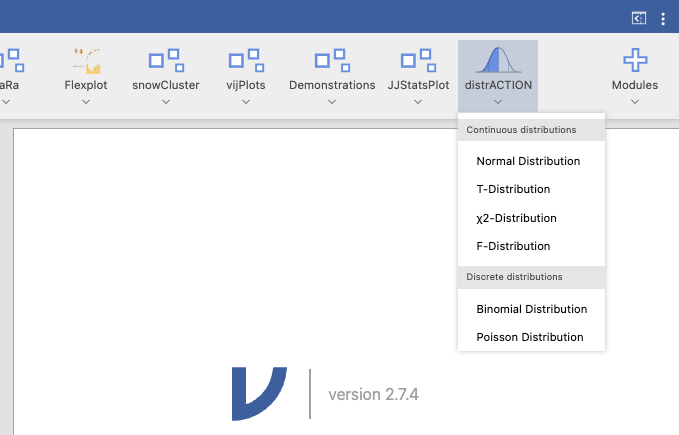
In Jamovi, you can install and use the external module called distrACTION to calculate probabilities for both Binomial and Poisson distributions.
Properties of a Continuous Probability Distribution
Let \(f(x)\) be a Probability Density Function (PDF). It must satisfy the following conditions:
\(f(x) \geq 0\) for all \(x\)
\(\int_{-\infty}^{\infty} f(x) \, dx = 1\)
The probability that \(X\) falls within the interval \(a \leq X \leq b\) is given by:
\[\begin{aligned} P(a < X < b) &= P(a \leq X < b) \\ &= P(a < X \leq b) \\ &= P(a \leq X \leq b) = \int_{a}^{b} f(x) \, dx \end{aligned}\]
Key Example
Normal Distribution
\[ f(x) = \frac{1}{\sigma \sqrt{2\pi}} e^{-\frac{(x - \mu)^2}{2\sigma^2}}, \quad \mu \in \mathbb{R},\ \sigma^2 > 0,\ x \in \mathbb{R} \]
\(\mu\) is the mean
\(\sigma^2\) is the variance
The shape is a bell curve (symmetrical)
Calculating the Probability in a Normal Distribution
import { Inputs, Plot } from "@observablehq/inputs"

// Input for mean (mu)
viewof mu = Inputs.range([-10, 10], { step: 0.1, value: 0, label: "Mean (μ)" })

// Input for standard deviation (sigma)
viewof sigma = Inputs.range([0.1, 10], { step: 0.1, value: 1, label: "Standard Deviation (σ)" })

// Input for a1 and a2
viewof a1 = Inputs.number({ label: "a₁", value: 0 })
viewof a2 = Inputs.number({ label: "a₂: (a₂ > a₁)", value: 1 })

// Selection of probability type
viewof probType = Inputs.select(["P(x < a₁)", "P(x > a₁)", "P(a₁ < x < a₂)"], { label: "Choose Probability Type" })
Important Continuous Probability Distributions
Normal Distribution:
Commonly used in statisticsUniform Distribution:
All values within a given interval have equal probabilityExponential Distribution:
Often used for modeling waiting times
Statistics
Statistics is the science of collecting, analyzing, interpreting, and presenting data to support decision-making or to better understand phenomena.
There are two main branches of statistics
1. Descriptive Statistics
Used to summarize and describe data, such as:
Mean
Median
Standard Deviation
Variance
Pearson Correlation
Frequency Table
Various types of charts and graphs (Previous chapter)
Mean or Average
Definition:
The mean, also known as the average, is a measure of central tendency that represents the typical value in a set of numbers.
\[\text{Mean} = \frac{\text{Sum of all values}}{\text{Number of values}}\]
\[\bar{x} = \frac{1}{n} \sum_{i=1}^{n} x_i\]
Where:
- \(\bar{x}\) = mean
- \(x_i\) = each individual value
- \(n\) = total number of values
How to Use the Mean
Summarizing Data
It gives a single value that represents the entire dataset.
Example: The average height of students in a class.
Comparing Groups
- You can compare the mean scores of two different classes or products.
- Used in Other Statistical Methods
Mean is the basis for calculating:
Variance and standard deviation
Z-scores
Regression analysis
Hypothesis testing
Example
Let’s say you have the following exam scores: 70, 80, 90, 85, 75
\[ \text{Mean} = \frac{70 + 80 + 90 + 85 + 75}{5} = \frac{400}{5} = 80 \]
So, the average score is 80.
When Not to Use the Mean
- Skewed data or outliers can distort the mean. In those cases, use the median (middle value) instead.
Median
Definition:
The median is the middle value of a dataset when the values are arranged in order. It divides the dataset into two equal halves.
If the number of data points is odd, the median is the middle number.
If the number is even, the median is the average of the two middle numbers.
How to Calculate the Median
Sort the data from smallest to largest.
Find the middle value:
If \(n\) is odd: \[\text{Median} = x_{(\frac{n+1}{2})}\]
If \(n\) is even: \[\text{Median} = \frac{x_{(n/2)} + x_{(n/2 + 1)}}{2}\]
How to Use the Median
Measure Central Tendency
- It shows the “typical” value, especially for skewed data.
When Data Has Outliers
- Unlike the mean, the median is not affected by extreme values.
Descriptive Statistics
- Used in summarizing income, house prices, ages, etc.
Example 1: Odd number of values
Data: 5, 7, 9
Sorted: 5, 7, 9
Median = 7 (the middle value)
Example 2: Even number of values
Data: 3, 5, 7, 9
Sorted: 3, 5, 7, 9
Median = (5 + 7) / 2 = 6
🥊 Mean vs. Median Battle
viewof outlierGame = (function() {
  const uid = "out_" + Math.random().toString(36).substr(2, 9);
  const width = 600;
  const height = 250;

  // Create container
  const container = html`<div style="font-family:'Sarabun', sans-serif; display:flex; flex-direction:column; align-items:center; gap:15px; background:white; padding:25px; border-radius:16px; border:1px solid #e2e8f0; box-shadow:0 4px 15px rgba(0,0,0,0.05); max-width:700px; margin:0 auto; user-select:none; -webkit-user-select:none;">
    <div style="font-size:14px; color:#64748b; text-align:center;">
      (Updated interaction) Try <b>pressing and dragging the red dot</b> to see how Mean and Median react.
    </div>

    <canvas width="${width}" height="${height}" style="width:100%; max-width:600px; height:auto; background:#f8fafc; border-radius:8px; border:1px solid #cbd5e1; cursor:ew-resize; touch-action:none;"></canvas>

    <div style="display:flex; gap:20px; width:100%; justify-content:center; flex-wrap:wrap;">
       <div style="text-align:center; padding:10px 20px; background:#dbeafe; border-radius:8px; color:#1e40af; min-width:140px;">
         <div style="font-size:12px;">Mean</div>
         <div id="${uid}-val-mean" style="font-size:24px; font-weight:bold;">0</div>
         <div style="font-size:10px;">(very sensitive)</div>
       </div>

       <div style="text-align:center; padding:10px 20px; background:#fce7f3; border-radius:8px; color:#9d174d; min-width:140px;">
         <div style="font-size:12px;">Median</div>
         <div id="${uid}-val-median" style="font-size:24px; font-weight:bold;">0</div>
         <div style="font-size:10px;">(more resistant)</div>
       </div>
    </div>
  </div>`;

  const canvas = container.querySelector("canvas");
  const ctx = canvas.getContext("2d");
  const elMean = container.querySelector(`#${uid}-val-mean`);
  const elMedian = container.querySelector(`#${uid}-val-median`);

  // Initial data
  let points = [100, 120, 130, 140, 150];
  let outlier = 160;
  let isDragging = false;
  let activePointerId = null;
  const Y_POS = height / 2;

  // Convert screen coordinates to canvas coordinates
  function getCanvasX(clientX) {
    const rect = canvas.getBoundingClientRect();
    const scaleX = canvas.width / rect.width;
    return (clientX - rect.left) * scaleX;
  }

  // Update values and redraw
  function update() {
    const allData = [...points, outlier].sort((a, b) => a - b);

    // Calculate mean
    const sum = allData.reduce((a, b) => a + b, 0);
    const mean = sum / allData.length;

    // Calculate median
    let median = 0;
    const mid = Math.floor(allData.length / 2);
    if (allData.length % 2 === 0) {
      median = (allData[mid - 1] + allData[mid]) / 2;
    } else {
      median = allData[mid];
    }

    elMean.innerText = mean.toFixed(1);
    elMedian.innerText = median.toFixed(1);
    draw(mean, median);
  }

  function draw(mean, median) {
    ctx.clearRect(0, 0, width, height);

    // Axis line
    ctx.beginPath();
    ctx.moveTo(20, Y_POS);
    ctx.lineTo(width - 20, Y_POS);
    ctx.strokeStyle = "#cbd5e1";
    ctx.lineWidth = 2;
    ctx.stroke();

    // Regular points (gray)
    ctx.fillStyle = "#94a3b8";
    points.forEach(p => {
      ctx.beginPath();
      ctx.arc(p, Y_POS, 6, 0, Math.PI * 2);
      ctx.fill();
    });

    // Outlier point (red) - larger for easier touch interaction
    ctx.fillStyle = "#ef4444";
    ctx.beginPath();
    ctx.arc(outlier, Y_POS, 12, 0, Math.PI * 2);
    ctx.fill();
    ctx.strokeStyle = "white";
    ctx.lineWidth = 2;
    ctx.stroke();

    // Mean line (blue, dashed)
    ctx.beginPath();
    ctx.moveTo(mean, Y_POS - 30);
    ctx.lineTo(mean, Y_POS + 30);
    ctx.strokeStyle = "#2563eb";
    ctx.lineWidth = 3;
    ctx.setLineDash([5, 3]);
    ctx.stroke();
    ctx.setLineDash([]);
    ctx.fillStyle = "#2563eb";
    ctx.font = "12px sans-serif";
    ctx.fillText("Mean", mean - 15, Y_POS - 35);

    // Median line (pink, solid)
    ctx.beginPath();
    ctx.moveTo(median, Y_POS - 20);
    ctx.lineTo(median, Y_POS + 20);
    ctx.strokeStyle = "#db2777";
    ctx.lineWidth = 3;
    ctx.stroke();
    ctx.fillStyle = "#db2777";
    ctx.fillText("Median", median - 22, Y_POS + 35);
  }

  // Start dragging
  canvas.addEventListener("pointerdown", (e) => {
    const x = getCanvasX(e.clientX);

    // Check whether the pointer is close to the red outlier
    if (Math.abs(x - outlier) < 30) {
      isDragging = true;
      activePointerId = e.pointerId;
      e.preventDefault();

      // Capture the pointer for smoother dragging
      if (canvas.setPointerCapture) {
        canvas.setPointerCapture(e.pointerId);
      }
    }
  });

  // Dragging
  canvas.addEventListener("pointermove", (e) => {
    if (!isDragging || e.pointerId !== activePointerId) return;
    e.preventDefault();

    let x = getCanvasX(e.clientX);

    // Keep the outlier inside the visible range
    if (x < 20) x = 20;
    if (x > width - 20) x = width - 20;

    outlier = x;
    update();
  });

  // End dragging
  function stopDragging(e) {
    if (activePointerId !== null && e.pointerId !== activePointerId) return;

    isDragging = false;

    if (canvas.releasePointerCapture && activePointerId !== null) {
      try {
        canvas.releasePointerCapture(activePointerId);
      } catch (err) {
        // Safe fallback
      }
    }

    activePointerId = null;
  }

  canvas.addEventListener("pointerup", stopDragging);
  canvas.addEventListener("pointercancel", stopDragging);

  // Initial draw
  update();
  return container;
})()
Variance
Definition:
Variance measures how much the values in a dataset differ from the mean. It tells us the spread or dispersion of the data.
A small variance means the data points are close to the mean.
A large variance means the data points are spread out over a wider range.
Formula
For a sample: \[s^2 = \frac{1}{n - 1} \sum_{i=1}^{n} (x_i - \bar{x})^2\] For a population: \[\sigma^2 = \frac{1}{N} \sum_{i=1}^{N} (x_i - \mu)^2\]
Where:
\(x_i\) = each data point
\(\bar{x}\) = sample mean
\(\mu\) = population mean
\(n\), \(N\) = number of values in the sample or population
\(s^2\), \(\sigma^2\) = variance
Example
Data: 4, 6, 8
Mean = (4 + 6 + 8) / 3 = 6
Deviations: -2, 0, +2
Squared deviations: 4, 0, 4
Variance (sample) = \(\frac{4 + 0 + 4}{3 - 1} = \frac{8}{2} = 4\)
How to Use Variance
Understand data spread
- Helps measure how consistent or variable the data is.
Compare variability
- Useful when comparing the performance or risk of different datasets or investments.
In statistics and machine learning. Variance is used in:
Standard deviation (√variance)
ANOVA
Regression analysis
Risk models in finance (Volatility)
Units of Variance
The unit of variance is the square of the original unit (e.g., if values are in meters, variance is in meters²).
That’s why standard deviation (the square root of variance) is often preferred for interpretation.
Standard Deviation
Definition:
The standard deviation is a measure of how spread out the values in a dataset are from the mean. It is the square root of the variance.
A low standard deviation means the data points are close to the mean.
A high standard deviation means the data points are more spread out.
Formula
For a sample: \[ s = \sqrt{\frac{1}{n - 1} \sum_{i=1}^{n} (x_i - \bar{x})^2} \] For a population: \[ \sigma = \sqrt{\frac{1}{N} \sum_{i=1}^{N} (x_i - \mu)^2} \]
Where:
\(x_i\) = each data value
\(\bar{x}\) = sample mean
\(\mu\) = population mean
\(s\), \(\sigma\) = standard deviation
\(n\), \(N\) = number of data points
Example
Data: 4, 6, 8
Mean = 6
Sample variance = \(\frac{(4-6)^2 + (6-6)^2 + (8-6)^2}{3 - 1} = 4\)
Standard deviation = \(\sqrt{4} = 2\)
How to Use Standard Deviation
Describe variability
- Shows how consistently data points are clustered around the mean.
Compare consistency
- Smaller standard deviation = more consistent results (e.g., test scores, product quality).
In statistical analysis Used in:
Confidence intervals
Hypothesis testing (e.g., z-tests, t-tests)
Control charts in quality control
Risk assessment in finance
Units of Standard Deviation
Same unit as the original data (e.g., if data is in cm, standard deviation is in cm).
This makes it more interpretable than variance.
Observing Data Distribution (Symmetry vs. Skewness)
Adjust the Skewness slider below to see how the Mean (solid red line) and Median (dashed blue line) separate as the distribution shifts away from symmetry:
Skewness (Left-skewed < 0 < Right-skewed):
data = {
  const raw = Array.from({length: sampleSize}, () => {
    const u1 = Math.random();
    const u2 = Math.random();
    const z0 = Math.sqrt(-2.0 * Math.log(u1)) * Math.cos(2.0 * Math.PI * u2);
    return z0;
  });

  return raw.map(x => {
    if (skewness === 0) return x * 10 + 50;
    if (skewness > 0) {
      return Math.pow(Math.abs(x), 1 + skewness * 0.3) * (x >= 0 ? 1 : -0.5) * 10 + 50;
    } else {
      const s = Math.abs(skewness);
      return -Math.pow(Math.abs(x), 1 + s * 0.3) * (x >= 0 ? -0.5 : 1) * 10 + 50;
    }
  });
}

// 3. Statistical Calculations
meanVal = d3.mean(data)
medianVal = d3.median(data)
sdVal = d3.deviation(data)
diffVal = Math.abs(meanVal - medianVal)
isSymmetric = diffVal < (0.2 * sdVal)

// 4. Kernel Density Estimation (KDE) Helper Functions
function epanechnikov(bandwidth) {
  return x => Math.abs(x /= bandwidth) <= 1 ? 0.75 * (1 - x * x) / bandwidth : 0;
}

function kde(kernel, thresholds, data) {
  return thresholds.map(t => [t, d3.mean(data, d => kernel(t - d))]);
}

// Generate Density points scaled to frequency counts for overlay
densityData = {
  const xMin = d3.min(data) - 10;
  const xMax = d3.max(data) + 10;
  const thresholds = d3.ticks(xMin, xMax, 100);
  const bw = 1.06 * sdVal * Math.pow(sampleSize, -0.2); // Silverman's rule of thumb
  const density = kde(epanechnikov(bw), thresholds, data);

  // Scale density height to match histogram frequency (bin width ≈ (xMax - xMin)/30)
  const binWidth = (xMax - xMin) / 30;
  return density.map(([x, y]) => ({ x, y: y * sampleSize * binWidth }));
}
// 5. Interactive Plot using Observable Plot
Plot.plot({
height: 400,
width: 700,
grid: true,
x: {label: "Value"},
y: {label: "Frequency / Density Scale"},
marks: [
// Histogram
Plot.rectY(
data,
Plot.binX({y: "count"}, {x: d => d, fill: "#cbd5e1", thresholds: 30})
),
// Density Curve Overlay (Orange Line)
Plot.line(densityData, {
x: "x",
y: "y",
stroke: "#f97316",
strokeWidth: 2
}),
// Rule for Mean (Red Solid Line)
Plot.ruleX([meanVal], {stroke: "#ef4444", strokeWidth: 3}),
Plot.text([meanVal], {
x: meanVal,
y: 0,
text: d => ` Mean: ${d.toFixed(2)}`,
fill: "#ef4444",
dy: -15,
textAnchor: "start",
fontWeight: "bold"
}),
// Rule for Median (Blue Dashed Line)
Plot.ruleX([medianVal], {stroke: "#0284c7", strokeWidth: 3, strokeDasharray: "4,4"}),
Plot.text([medianVal], {
x: medianVal,
y: 0,
text: d => ` Median: ${d.toFixed(2)}`,
fill: "#0284c7",
dy: -35,
textAnchor: "start",
fontWeight: "bold"
})
]
})// ใช้ html tag เพื่อประมวลผลตัวแปร OJS ออกมาเป็นตัวเลขจริง
html`<div class="callout callout-style-default callout-note callout-titled">
<div class="callout-header d-flex align-content-center">
<div class="callout-icon-container">
<i class="callout-icon"></i>
</div>
<div class="callout-title-container flex-fill">
📊 Summary Statistics
</div>
</div>
<div class="callout-body-container callout-body">
<ul>
<li><b>Mean:</b> ${meanVal.toFixed(2)}</li>
<li><b>Median:</b> ${medianVal.toFixed(2)}</li>
<li><b>|Mean - Median|:</b> ${diffVal.toFixed(2)} (${(diffVal / sdVal).toFixed(2)} SD)</li>
<li><b>Symmetry Status (Rule of Thumb < 0.2 SD):</b>
<span style="color: ${isSymmetric ? '#16a34a' : '#dc2626'}; font-weight: bold;">
${isSymmetric ? "Symmetric Distribution" : "Asymmetric / Skewed Distribution"}
</span>
</li>
</ul>
</div>
</div>`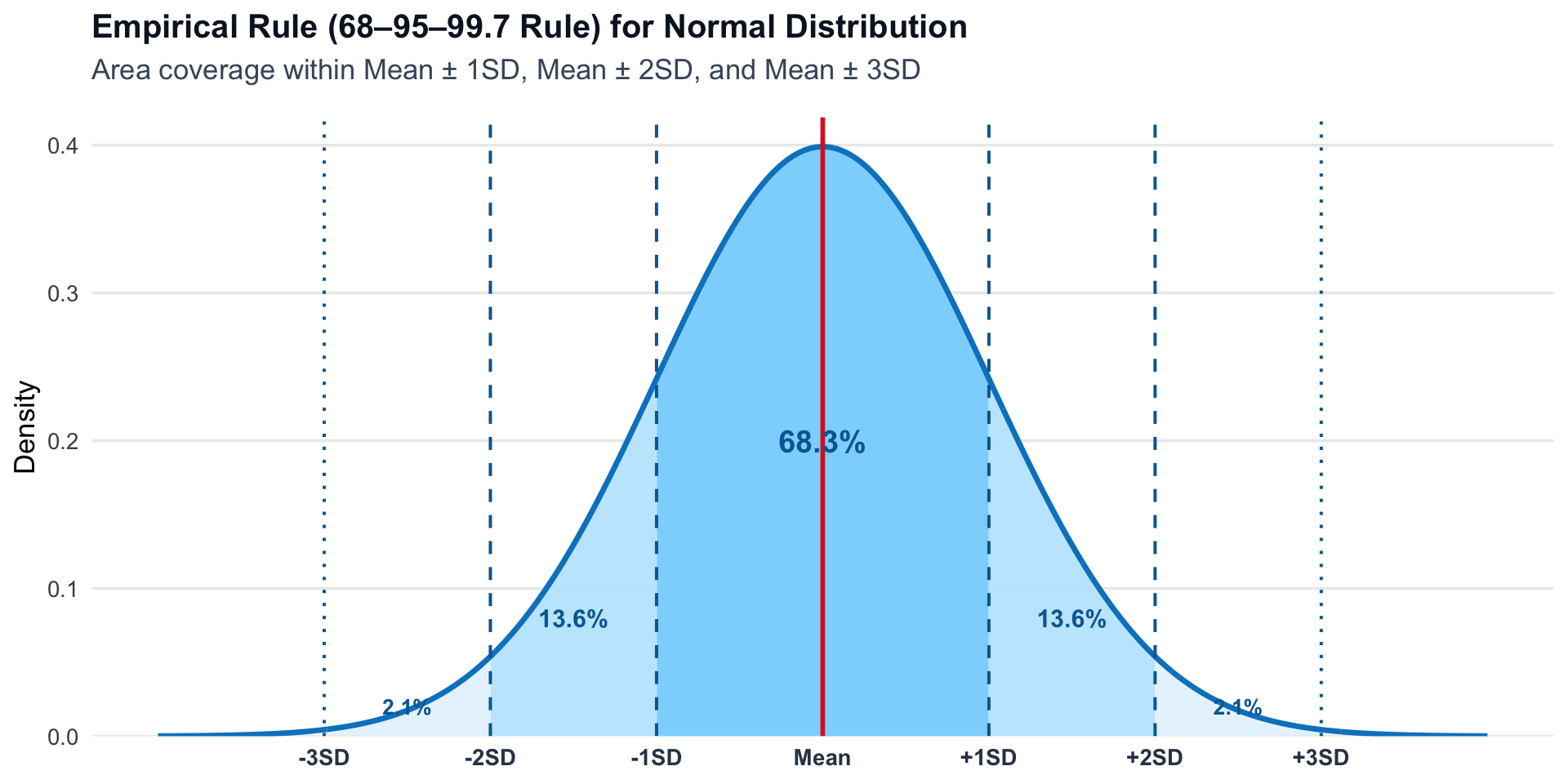
Interactive Normal Distribution & Empirical Rule Checker”
Interactive Normality & Outlier Inspection
Adjust the controls below to simulate data with different skewness levels and extreme outliers:
- Skewness Level:
- Contaminate with Outliers (%):
norm_data = {
  const numOutliers = Math.round((norm_sampleN * norm_outlierPct) / 100);
  const numNormal = norm_sampleN - numOutliers;

  // Generate main distribution
  const raw = Array.from({length: numNormal}, () => {
    const u1 = Math.random();
    const u2 = Math.random();
    return Math.sqrt(-2.0 * Math.log(u1)) * Math.cos(2.0 * Math.PI * u2);
  });

  const mainData = raw.map(x => {
    if (norm_skew === 0) return x * 10 + 50;
    if (norm_skew > 0) {
      return Math.pow(Math.abs(x), 1 + norm_skew * 0.3) * (x >= 0 ? 1 : -0.5) * 10 + 50;
    } else {
      const s = Math.abs(norm_skew);
      return -Math.pow(Math.abs(x), 1 + s * 0.3) * (x >= 0 ? -0.5 : 1) * 10 + 50;
    }
  });

  // Inject Extreme Outliers (placed beyond +4 SD)
  const outliers = Array.from({length: numOutliers}, () => {
    return 50 + 40 + (Math.random() * 20);
  });

  return [...mainData, ...outliers];
}

// 3. Statistical Metrics
norm_meanVal = d3.mean(norm_data)
norm_medianVal = d3.median(norm_data)
norm_sdVal = d3.deviation(norm_data)
norm_diffVal = Math.abs(norm_meanVal - norm_medianVal)

// Symmetry Rule Check (< 0.2 SD)
norm_isSymmetric = norm_diffVal < (0.2 * norm_sdVal)

// Empirical Rule Coverage Calculations
norm_count1SD = norm_data.filter(d => Math.abs(d - norm_meanVal) <= 1 * norm_sdVal).length
norm_count2SD = norm_data.filter(d => Math.abs(d - norm_meanVal) <= 2 * norm_sdVal).length
norm_count3SD = norm_data.filter(d => Math.abs(d - norm_meanVal) <= 3 * norm_sdVal).length

norm_pct1SD = (norm_count1SD / norm_sampleN) * 100
norm_pct2SD = (norm_count2SD / norm_sampleN) * 100
norm_pct3SD = (norm_count3SD / norm_sampleN) * 100

// Outlier Count (> 3 SD)
norm_outliersBeyond3SD = norm_sampleN - norm_count3SD
// 4. Interactive Visualization with SD Bands
Plot.plot({
height: 420,
width: 720,
grid: true,
x: {label: "Value"},
y: {label: "Count"},
marks: [
// Histogram
Plot.rectY(
norm_data,
Plot.binX({y: "count"}, {x: d => d, fill: "#e2e8f0", stroke: "#cbd5e1", thresholds: 35})
),
// SD Coverage Shading Bands
Plot.rectX([[norm_meanVal - 3 * norm_sdVal, norm_meanVal + 3 * norm_sdVal]], {fill: "#fef08a", opacity: 0.15}),
Plot.rectX([[norm_meanVal - 2 * norm_sdVal, norm_meanVal + 2 * norm_sdVal]], {fill: "#bbf7d0", opacity: 0.25}),
Plot.rectX([[norm_meanVal - 1 * norm_sdVal, norm_meanVal + 1 * norm_sdVal]], {fill: "#bfdbfe", opacity: 0.35}),
// SD Boundaries Lines (±1SD, ±2SD, ±3SD)
Plot.ruleX([norm_meanVal - 1 * norm_sdVal, norm_meanVal + 1 * norm_sdVal], {stroke: "#3b82f6", strokeDasharray: "2,2"}),
Plot.ruleX([norm_meanVal - 2 * norm_sdVal, norm_meanVal + 2 * norm_sdVal], {stroke: "#22c55e", strokeDasharray: "2,2"}),
Plot.ruleX([norm_meanVal - 3 * norm_sdVal, norm_meanVal + 3 * norm_sdVal], {stroke: "#eab308", strokeDasharray: "2,2"}),
// Mean Line (Red)
Plot.ruleX([norm_meanVal], {stroke: "#ef4444", strokeWidth: 2.5}),
Plot.text([norm_meanVal], {
x: norm_meanVal,
y: 0,
text: d => ` Mean: ${d.toFixed(2)}`,
fill: "#ef4444",
dy: -15,
textAnchor: "start",
fontWeight: "bold"
}),
// Median Line (Blue)
Plot.ruleX([norm_medianVal], {stroke: "#0284c7", strokeWidth: 2.5, strokeDasharray: "4,4"}),
Plot.text([norm_medianVal], {
x: norm_medianVal,
y: 0,
text: d => ` Median: ${d.toFixed(2)}`,
fill: "#0284c7",
dy: -35,
textAnchor: "start",
fontWeight: "bold"
})
]
})// 5. Dynamic Summary Cards using OJS html Tag
html`<div class="callout callout-style-default callout-note callout-titled">
<div class="callout-header d-flex align-content-center">
<div class="callout-icon-container"><i class="callout-icon"></i></div>
<div class="callout-title-container flex-fill">📊 Normality & Empirical Rule Check Results</div>
</div>
<div class="callout-body-container callout-body">
<h5>1. Symmetry Test (|Mean - Median| < 0.2 SD)</h5>
<ul>
<li><b>Mean:</b> ${norm_meanVal.toFixed(2)} | <b>Median:</b> ${norm_medianVal.toFixed(2)}</li>
<li><b>|Mean - Median|:</b> ${norm_diffVal.toFixed(2)} (Threshold = ${(0.2 * norm_sdVal).toFixed(2)} SD)</li>
<li><b>Status:</b>
<span style="color: ${norm_isSymmetric ? '#16a34a' : '#dc2626'}; font-weight: bold;">
${norm_isSymmetric ? "✓ Pass (Symmetric Distribution)" : "✗ Fail (Asymmetric / Skewed Distribution)"}
</span>
</li>
</ul>
<h5>2. Empirical Rule Coverage (68% - 95% - 99.7% Rule)</h5>
<table class="table table-sm" style="max-width: 550px;">
<thead>
<tr>
<th>Interval</th>
<th>Observed Coverage</th>
<th>Expected (Normal)</th>
<th>Status</th>
</tr>
</thead>
<tbody>
<tr>
<td><b>Mean ± 1 SD</b></td>
<td>${norm_pct1SD.toFixed(1)}%</td>
<td>~68.3%</td>
<td>${Math.abs(norm_pct1SD - 68.3) < 4 ? "✓ Normal" : "⚠ Deviated"}</td>
</tr>
<tr>
<td><b>Mean ± 2 SD</b></td>
<td>${norm_pct2SD.toFixed(1)}%</td>
<td>~95.5%</td>
<td>${Math.abs(norm_pct2SD - 95.5) < 3 ? "✓ Normal" : "⚠ Deviated"}</td>
</tr>
<tr>
<td><b>Mean ± 3 SD</b></td>
<td>${norm_pct3SD.toFixed(1)}%</td>
<td>~99.7%</td>
<td>${norm_pct3SD >= 98.5 ? "✓ Normal" : "⚠ Deviated"}</td>
</tr>
</tbody>
</table>
<h5>3. Extreme Outlier Check (> Mean ± 3 SD)</h5>
<ul>
<li><b>Outliers Detected:</b> ${norm_outliersBeyond3SD} points (${((norm_outliersBeyond3SD / norm_sampleN) * 100).toFixed(1)}% of dataset)</li>
<li><b>Interpretation:</b> ${norm_outliersBeyond3SD === 0 ? "No extreme outliers found." : `Found ${norm_outliersBeyond3SD} potential extreme outlier(s) pulling the Mean.`}</li>
</ul>
</div>
</div>`📊 Distribution Lab (Beta Distribution)
viewof betaDistCorrected = (function() {
  const uid = "beta_fixed_" + Math.random().toString(36).substr(2, 9);
  const width = 700;
  const height = 400;

  const container = html`<div style="font-family:'Sarabun', sans-serif; display:flex; flex-direction:column; align-items:center; gap:15px; background:white; padding:20px; border-radius:16px; border:1px solid #e2e8f0; box-shadow:0 4px 15px rgba(0,0,0,0.05); max-width:750px; margin:0 auto;">
    <div style="font-size:13px; color:#64748b; text-align:center;">
      Adjust Alpha and Beta to observe changes in skewness and kurtosis
    </div>

    <div style="position:relative;">
      <canvas width="${width}" height="${height}" style="background:#f8fafc; border-radius:8px; border:1px solid #cbd5e1;"></canvas>

      <div style="position:absolute; top:10px; right:10px; background:rgba(255,255,255,0.95); padding:10px; border-radius:8px; border:1px solid #94a3b8; font-size:12px; box-shadow:0 2px 10px rgba(0,0,0,0.1);">
        <div style="margin-bottom:5px; font-weight:bold; color:#1e293b; border-bottom:1px solid #e2e8f0; padding-bottom:3px;">Statistics Legend</div>

        <div style="display:grid; grid-template-columns: auto auto; gap:3px 10px;">
           <div style="color:#dc2626; font-weight:bold;">Mean:</div>
           <div id="${uid}-val-mean" style="text-align:right;">-</div>

           <div style="color:#2563eb; font-weight:bold;">Median:</div>
           <div id="${uid}-val-median" style="text-align:right;">-</div>

           <div style="color:#059669;">SD:</div>
           <div id="${uid}-val-sd" style="text-align:right;">-</div>

           <div style="color:#7c3aed; font-weight:bold;">Skewness:</div>
           <div id="${uid}-val-skew" style="text-align:right; font-weight:bold; color:#7c3aed;">-</div>

           <div style="color:#db2777; font-weight:bold;">Kurtosis:</div>
           <div id="${uid}-val-kurt" style="text-align:right; font-weight:bold; color:#db2777;">-</div>
        </div>
      </div>
    </div>

    <div style="width:100%; display:grid; grid-template-columns: 1fr 1fr; gap:15px; background:#f1f5f9; padding:15px; border-radius:12px;">

       <div>
         <div style="display:flex; justify-content:space-between; align-items:center; margin-bottom:2px;">
            <span style="font-weight:bold; color:#334155; font-size:12px; white-space:nowrap;">Parameter α (Alpha)</span>
            <span id="${uid}-disp-a" style="font-weight:bold; color:#2563eb; font-size:12px;">2.0</span>
         </div>
         <input id="${uid}-sl-a" type="range" min="0.5" max="10" value="2" step="0.1" style="width:100%; accent-color:#4338ca; margin:5px 0;">
         <div style="font-size:10px; color:#64748b; white-space:nowrap;">(Smaller values push the distribution toward the left/boundary)</div>
       </div>

       <div>
         <div style="display:flex; justify-content:space-between; align-items:center; margin-bottom:2px;">
            <span style="font-weight:bold; color:#334155; font-size:12px; white-space:nowrap;">Parameter β (Beta)</span>
            <span id="${uid}-disp-b" style="font-weight:bold; color:#ea580c; font-size:12px;">5.0</span>
         </div>
         <input id="${uid}-sl-b" type="range" min="0.5" max="10" value="5" step="0.1" style="width:100%; accent-color:#4338ca; margin:5px 0;">
         <div style="font-size:10px; color:#64748b; white-space:nowrap;">(Smaller values push the distribution toward the right/boundary)</div>
       </div>
    </div>

  </div>`;

  const canvas = container.querySelector("canvas");
  const ctx = canvas.getContext("2d");

  const slA = container.querySelector(`#${uid}-sl-a`);
  const slB = container.querySelector(`#${uid}-sl-b`);
  const dispA = container.querySelector(`#${uid}-disp-a`);
  const dispB = container.querySelector(`#${uid}-disp-b`);

  const elMean = container.querySelector(`#${uid}-val-mean`);
  const elMedian = container.querySelector(`#${uid}-val-median`);
  const elSD = container.querySelector(`#${uid}-val-sd`);
  const elSkew = container.querySelector(`#${uid}-val-skew`);
  const elKurt = container.querySelector(`#${uid}-val-kurt`);

  function logGamma(z) {
    const c = [
      57.1562356658629235,
      -59.5979603554754912,
      14.1360979747417471,
      -0.491913816097620199,
      .339946499848118887e-4,
      .465236289270485756e-4,
      -.980110293032623307e-5,
      .158088703224912494e-3,
      -.249910353874351101e-2,
      .177454516771575316e-1,
      .754705354271336459,
      .252012282494909806
    ];

    let sum = c[0];

    for (let i = 1; i < c.length; i++) {
      sum += c[i] / (z + i);
    }

    let g = (z + 0.5) * Math.log(z + 5.5) - (z + 5.5);

    return g + Math.log(2.5066282746310005 * sum / z);
  }

  function betaPDF(x, a, b) {
    if (x <= 0 || x >= 1) return 0;

    const lnVal =
      logGamma(a + b) -
      logGamma(a) -
      logGamma(b) +
      (a - 1) * Math.log(x) +
      (b - 1) * Math.log(1 - x);

    return Math.exp(lnVal);
  }

  function update() {
    const a = parseFloat(slA.value);
    const b = parseFloat(slB.value);

    dispA.innerText = a.toFixed(1);
    dispB.innerText = b.toFixed(1);

    const mean = a / (a + b);

    const variance =
      (a * b) /
      (Math.pow(a + b, 2) * (a + b + 1));

    const sd = Math.sqrt(variance);

    // Skewness
    let skew = 0;

    if (a !== b) {
      skew =
        (2 * (b - a) * Math.sqrt(a + b + 1)) /
        ((a + b + 2) * Math.sqrt(a * b));
    }

    // Kurtosis
    const num =
      6 *
      (
        Math.pow(a - b, 2) * (a + b + 1) -
        (a * b * (a + b + 2))
      );

    const den =
      a * b * (a + b + 2) * (a + b + 3);

    const kurt = num / den;

    // Accurate median approximation
    // Groeneveld & Meeden (1977)
    const median =
      (a - 1 / 3) /
      (a + b - 2 / 3);

    const scale = 100;

    elMean.innerText = (mean * scale).toFixed(2);
    elMedian.innerText = (median * scale).toFixed(2);
    elSD.innerText = (sd * scale).toFixed(2);
    elSkew.innerText = skew.toFixed(3);
    elKurt.innerText = kurt.toFixed(3);

    if (skew > 0.1) {
      elSkew.style.color = "#ea580c";
    } else if (skew < -0.1) {
      elSkew.style.color = "#dc2626";
    } else {
      elSkew.style.color = "#16a34a";
    }

    // Draw the graph
    ctx.clearRect(0, 0, width, height);

    const pad = 40;
    const drawW = width - pad * 2;
    const drawH = height - pad * 2;

    let maxY = 0;
    let points = [];

    for (let i = 0; i <= drawW; i++) {
      const x = i / drawW;

      const safeX =
        Math.max(0.001, Math.min(0.999, x));

      const y = betaPDF(safeX, a, b);

      if (y > maxY) {
        maxY = y;
      }

      points.push({
        x: safeX,
        y: y
      });
    }

    if (maxY > 10) {
      maxY = 10;
    }

    // Draw the shaded area under the curve
    ctx.beginPath();
    ctx.moveTo(pad, height - pad);

    points.forEach((p) => {
      const plotX = pad + (p.x * drawW);

      const plotY =
        (height - pad) -
        (p.y / maxY * drawH);

      ctx.lineTo(plotX, plotY);
    });

    ctx.lineTo(pad + drawW, height - pad);

    ctx.fillStyle = "rgba(99, 102, 241, 0.2)";
    ctx.fill();

    // Draw the probability density curve
    ctx.beginPath();

    points.forEach((p, i) => {
      const plotX = pad + (p.x * drawW);

      const plotY =
        (height - pad) -
        (p.y / maxY * drawH);

      if (i === 0) {
        ctx.moveTo(plotX, plotY);
      } else {
        ctx.lineTo(plotX, plotY);
      }
    });

    ctx.lineWidth = 3;
    ctx.strokeStyle = "#4f46e5";
    ctx.stroke();

    const drawLine = (val, color, label) => {
      // Clamp the value between 0 and 1
      const safeVal =
        Math.max(0, Math.min(1, val));

      const xPos =
        pad + (safeVal * drawW);

      ctx.beginPath();
      ctx.moveTo(xPos, pad);
      ctx.lineTo(xPos, height - pad);

      ctx.strokeStyle = color;
      ctx.lineWidth = 2;

      ctx.setLineDash(
        label === "Median" ? [] : [5, 5]
      );

      ctx.stroke();
      ctx.setLineDash([]);

      ctx.fillStyle = color;
      ctx.font = "bold 12px sans-serif";

      ctx.fillText(
        label,
        xPos - 15,
        height - pad + 15
      );

      const yAtVal = betaPDF(
        Math.max(
          0.001,
          Math.min(0.999, safeVal)
        ),
        a,
        b
      );

      const safeY =
        Math.min(yAtVal, maxY);

      const yPos =
        (height - pad) -
        (safeY / maxY * drawH);

      ctx.beginPath();
      ctx.arc(
        xPos,
        yPos,
        5,
        0,
        Math.PI * 2
      );

      ctx.fill();
    };

    drawLine(
      mean,
      "#dc2626",
      "Mean"
    );

    drawLine(
      median,
      "#2563eb",
      "Median"
    );

    // Draw the horizontal axis
    ctx.beginPath();
    ctx.moveTo(pad, height - pad);
    ctx.lineTo(width - pad, height - pad);

    ctx.strokeStyle = "#334155";
    ctx.lineWidth = 1;
    ctx.stroke();
  }

  slA.oninput = update;
  slB.oninput = update;

  update();

  return container;
})()
Pearson Correlation
Definition:
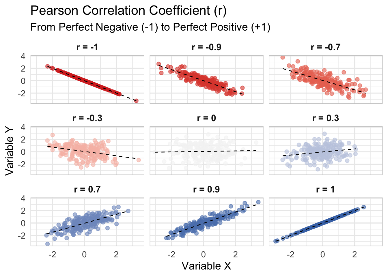
The Pearson correlation coefficient (denoted as \(r\)) measures the strength and direction of the linear relationship between two numerical variables.
- Values range from –1 to +1.
Formula:
\[ r = \frac{\sum (x_i - \bar{x})(y_i - \bar{y})}{\sqrt{\sum (x_i - \bar{x})^2} \cdot \sqrt{\sum (y_i - \bar{y})^2}} \]
Where:
\(x_i, y_i\) = values of the two variables
\(\bar{x}, \bar{y}\) = means of each variable
Example:
Imagine you collect data on students’ study time (hours) and exam scores:
| Study Time (X) | Exam Score (Y) |
|---|---|
| 1 | 50 |
| 2 | 60 |
| 3 | 70 |
| 4 | 80 |
| 5 | 90 |
The Pearson correlation would be +1, showing a perfect positive linear relationship.
Interpretation of \(r\):
| \(r\) value | Interpretation |
|---|---|
| \(+1\) | Perfect positive linear correlation |
| \(0.7\) to \(0.9\) | Strong positive linear correlation |
| \(0.3\) to \(0.7\) | Moderate positive linear correlation |
| \(0\) | No linear correlation |
| \(-0.3\) to \(-0.7\) | Moderate negative linear correlation |
| \(-0.7\) to \(-0.9\) | Strong negative linear correlation |
| \(-1\) | Perfect negative linear correlation |
How to Use Pearson Correlation
Measure Relationships
- To assess how strongly two variables are related (e.g., height and weight, income and spending).
Feature Selection
- In machine learning, to eliminate highly correlated predictors (multicollinearity).
Hypothesis Testing
- You can test whether the correlation is significantly different from zero using a t-test.
When Not to Use Pearson Correlation
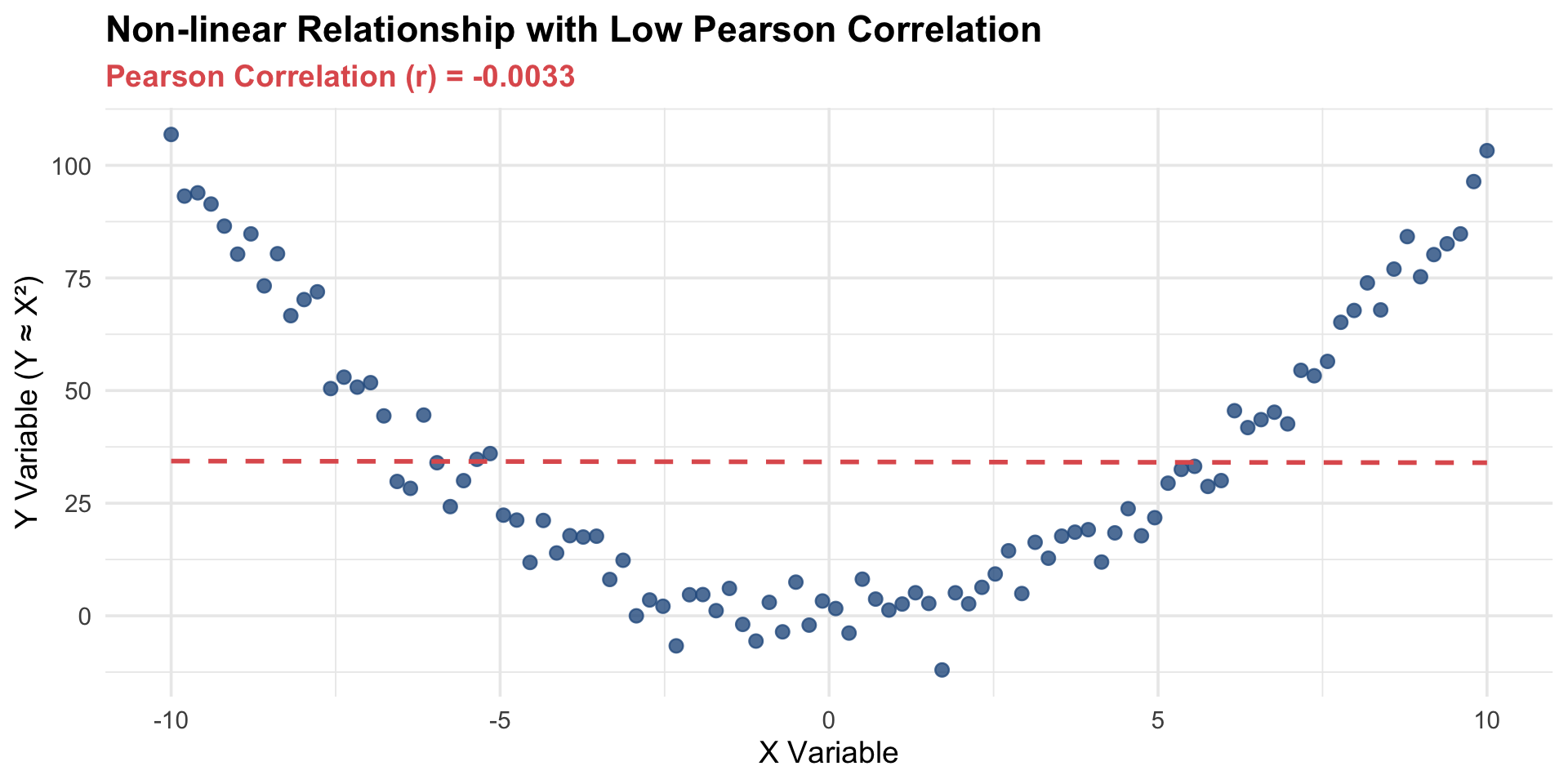
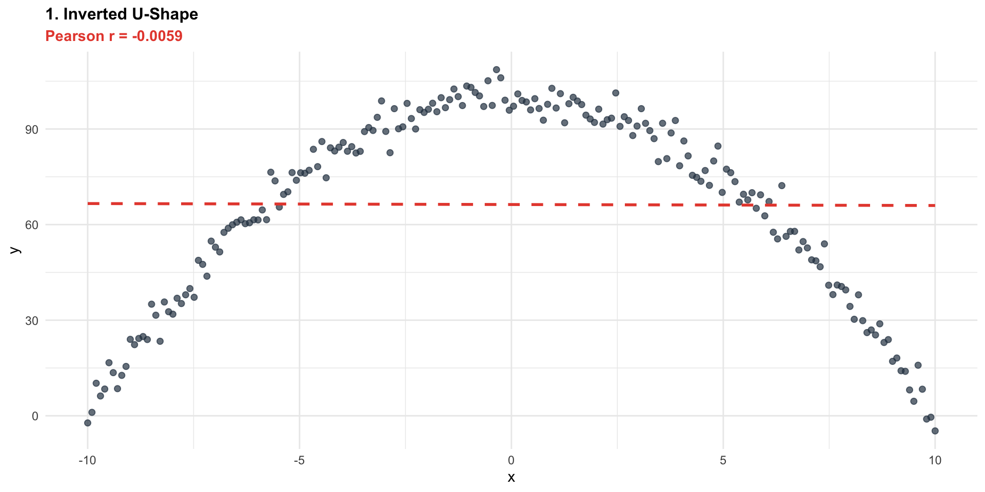
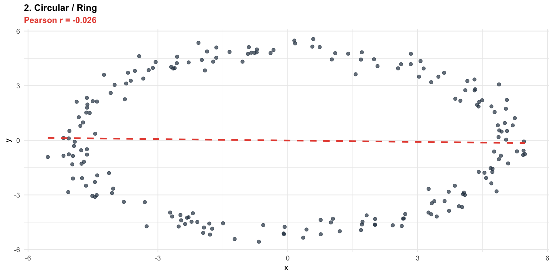
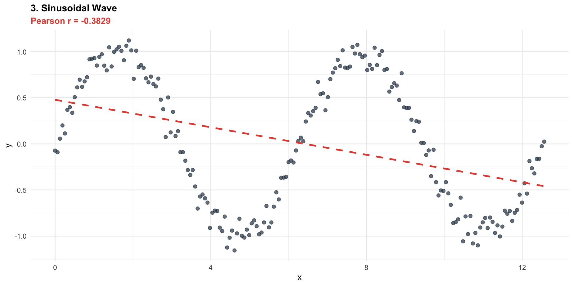
When the relationship is nonlinear.
When the data is not normally distributed.
When variables are ordinal or categorical (use Spearman or Kendall’s correlation instead).
Pearson Correlation:
Used to measure the linear relationship between two variables (\(r\)).
| \(r\) value | Meaning |
|---|---|
| +1 | Perfect positive correlation |
| 0 | No linear correlation |
| -1 | Perfect negative correlation |
Non-linear correlation
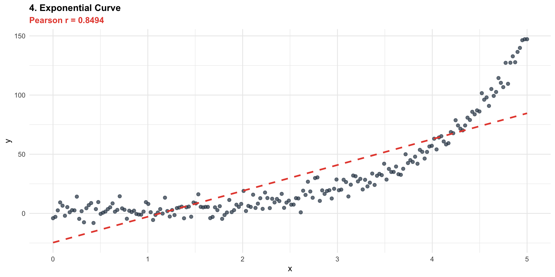
Anscombe’s Quartet: Same Statistics, Different Stories
Select Data:
Statistical Summary
| Stat | Value |
|---|---|
| Mean X | |
| Mean Y | |
| Corr. | 0.816 |
Plot.plot({
  height: 550, // ปรับความสูงให้พอดีสไลด์
  width: 700,
  grid: true,
  marks: [
    Plot.linearRegressionY(filtered, {x: "x", y: "y", stroke: "red", strokeWidth: 4}),
    Plot.dot(filtered, {x: "x", y: "y", fill: "steelblue", r: 10}),
    Plot.ruleX([0]),
    Plot.ruleY([0])
  ],
  x: {domain: [0, 20], label: "Variable X"},
  y: {domain: [0, 14], label: "Variable Y"},
  style: {fontSize: "18px", backgroundColor: "white"}
})
💡 Real-Life Examples of Correlation
“The more…, the more…”
- 📚 Study time ⬆️ → Exam scores ⬆️
- 📏 Height ⬆️ → Weight ⬆️
- 🌡️ Temperature ⬆️ → 🍦 Ice cream sales ⬆️
“The more…, the less…”
- 🚗 Driving speed ⬆️ → ⏱️ Travel time ⬇️
- 💰 Product price ⬆️ → 🛒 Sales ⬇️
- 🏫 Class absences ⬆️ → 🎓 GPA ⬇️
“No relationship”
- 👟 Shoe size ↔︎️ 🧠 Intelligence (IQ)
- 🪙 Gold price ↔︎️ 🌧️ Rainfall
- 🪪 National ID number ↔︎️ 📝 Grades
2. Inferential Statistics
Used to analyze data in order to draw conclusions or make predictions about a population, based on a sample.
Hypothesis Testing
Parameter Estimation
Regression Analysis
Applications of Statistics
1. Business and Marketing
Analyze market trends and customer behavior
Forecast product sales using Time Series Analysis
Use A/B Testing to compare the effectiveness of advertisements or marketing campaigns
2. Economics and Finance
Analyze economic conditions, such as calculating inflation and unemployment rates
Assess risk and return in investment portfolios (Portfolio Analysis)
Use econometric models to study factors influencing the economy
3. Science and Engineering
Design experiments (Design of Experiments) to develop new products
Analyze data from experiments in physics, chemistry, and biology
Perform quality control using Statistical Quality Control (SQC)
4. Medicine and Public Health
Analyze the effects of drugs or vaccines using Biostatistics
Study disease risks through Epidemiological data analysis
Use Machine Learning and AI to analyze medical records and assist in diagnosis
5. Data Science and Artificial Intelligence (AI)
Analyze Big Data to gain insights for data-driven decision making
Use Machine Learning techniques to develop predictive models
Perform Text Mining and analyze social media data
6. Education and Research
Analyze students’ academic performance and evaluate the effectiveness of curricula
Use statistics to design research studies that yield reliable conclusions
Analyze experimental data to test scientific hypotheses
Mean-Variance Criteria
This refers to a decision-making framework used in finance, economics, and statistics, especially in portfolio selection and investment analysis. It is based on the ideas introduced by Harry Markowitz in his Modern Portfolio Theory (MPT).
Definition:
The Mean-Variance Criteria evaluates and compares alternatives (such as portfolios, investment strategies, or decisions) based on two key factors:
Mean = expected return (reward)
Variance = risk (volatility of return)
We prefer a high average and a low variance.
Decision Rule (Mean-Variance Dominance):
Given two choices A and B:
A is preferred over B if:
- \(\mu_A \geq \mu_B\) and
- \(\sigma^2_A \leq \sigma^2_B\),
- with at least one strict inequality.
This means that A has higher or equal return and lower or equal risk than B.
In another case, it means we are unable to make a decision.
Example
| Option | Mean (Return) | Variance (Risk) |
|---|---|---|
| A | 8% | 4 |
| B | 7% | 5 |
| C | 9% | 6 |
A dominates B (higher return and lower risk) → eliminate B
A vs. C: A = safer, C = more profitable → Choice depends on risk tolerance
💼 Mean–Variance Decision Simulator
viewof mvGame = (function() {
  const uid = "mv_" + Math.random().toString(36).substr(2, 9);
  const width = 700;
  const height = 350;

  const container = html`<div style="
    font-family:'Sarabun', sans-serif;
    display:flex;
    flex-direction:column;
    align-items:center;
    gap:20px;
    background:white;
    padding:25px;
    border-radius:16px;
    border:1px solid #e2e8f0;
    box-shadow:0 4px 15px rgba(0,0,0,0.05);
    max-width:750px;
    margin:0 auto;">

    <div style="font-size:14px; color:#64748b; text-align:center;">
      Compare two investments using the <b>Mean–Variance Criterion</b>:
      prefer a <b>higher mean return</b> and a <b>lower variance</b>.
    </div>

    <div style="position:relative; width:100%;">
      <canvas
        width="${width}"
        height="${height}"
        style="
          width:100%;
          max-width:700px;
          height:auto;
          background:#f8fafc;
          border-radius:8px;
          border:1px solid #cbd5e1;">
      </canvas>

      <div style="
        position:absolute;
        bottom:5px;
        right:10px;
        font-size:12px;
        color:#64748b;">
        Return (%) ➡️
      </div>
    </div>

    <div style="
      width:100%;
      display:grid;
      grid-template-columns:1fr 1fr;
      gap:20px;
      background:#f1f5f9;
      padding:15px;
      border-radius:12px;">

      <!-- Fund A -->
      <div style="border-right:1px solid #cbd5e1; padding-right:15px;">
        <div style="
          color:#2563eb;
          font-weight:bold;
          margin-bottom:10px;
          white-space:nowrap;">
          🔵 Fund A
        </div>

        <div style="display:flex; justify-content:space-between; font-size:12px;">
          <span>
            Mean Return:
            <b id="${uid}-val-ma">8</b>%
          </span>
        </div>

        <input
          id="${uid}-sl-ma"
          type="range"
          min="0"
          max="25"
          value="8"
          step="0.5"
          style="width:100%; accent-color:#2563eb;">

        <div style="
          display:flex;
          justify-content:space-between;
          font-size:12px;
          margin-top:8px;">
          <span>
            Standard Deviation:
            <b id="${uid}-val-sa">2</b>%
          </span>
        </div>

        <input
          id="${uid}-sl-sa"
          type="range"
          min="1"
          max="10"
          value="2"
          step="0.5"
          style="width:100%; accent-color:#2563eb;">
      </div>

      <!-- Fund B -->
      <div style="padding-left:5px;">
        <div style="
          color:#ea580c;
          font-weight:bold;
          margin-bottom:10px;
          white-space:nowrap;">
          🟠 Fund B
        </div>

        <div style="display:flex; justify-content:space-between; font-size:12px;">
          <span>
            Mean Return:
            <b id="${uid}-val-mb">12</b>%
          </span>
        </div>

        <input
          id="${uid}-sl-mb"
          type="range"
          min="0"
          max="25"
          value="12"
          step="0.5"
          style="width:100%; accent-color:#ea580c;">

        <div style="
          display:flex;
          justify-content:space-between;
          font-size:12px;
          margin-top:8px;">
          <span>
            Standard Deviation:
            <b id="${uid}-val-sb">5</b>%
          </span>
        </div>

        <input
          id="${uid}-sl-sb"
          type="range"
          min="1"
          max="10"
          value="5"
          step="0.5"
          style="width:100%; accent-color:#ea580c;">
      </div>
    </div>

    <!-- Summary Cards -->
    <div style="display:flex; gap:15px; width:100%; flex-wrap:wrap;">

      <div id="${uid}-card-a" style="
        flex:1;
        min-width:220px;
        padding:15px;
        border-radius:12px;
        border:2px solid #e2e8f0;
        text-align:center;
        transition:0.3s;">

        <div style="font-size:14px; font-weight:bold; color:#2563eb;">
          🔵 Fund A
        </div>

        <div style="font-size:13px; color:#64748b; margin-top:8px;">
          Mean Return
        </div>

        <div id="${uid}-mean-a" style="
          font-size:21px;
          font-weight:bold;
          color:#2563eb;">
          0%
        </div>

        <div style="font-size:13px; color:#64748b; margin-top:6px;">
          Variance
        </div>

        <div id="${uid}-var-a" style="
          font-size:21px;
          font-weight:bold;
          color:#2563eb;">
          0
        </div>
      </div>

      <div id="${uid}-card-b" style="
        flex:1;
        min-width:220px;
        padding:15px;
        border-radius:12px;
        border:2px solid #e2e8f0;
        text-align:center;
        transition:0.3s;">

        <div style="font-size:14px; font-weight:bold; color:#ea580c;">
          🟠 Fund B
        </div>

        <div style="font-size:13px; color:#64748b; margin-top:8px;">
          Mean Return
        </div>

        <div id="${uid}-mean-b" style="
          font-size:21px;
          font-weight:bold;
          color:#ea580c;">
          0%
        </div>

        <div style="font-size:13px; color:#64748b; margin-top:6px;">
          Variance
        </div>

        <div id="${uid}-var-b" style="
          font-size:21px;
          font-weight:bold;
          color:#ea580c;">
          0
        </div>
      </div>

    </div>

    <!-- Decision -->
    <div id="${uid}-winner" style="
      width:100%;
      padding:15px;
      box-sizing:border-box;
      border-radius:12px;
      background:#f8fafc;
      border:1px solid #e2e8f0;
      font-size:16px;
      font-weight:bold;
      text-align:center;
      min-height:55px;">
    </div>

    <div style="
      font-size:12px;
      color:#64748b;
      width:100%;
      line-height:1.5;">

      <b>Mean–Variance Criterion:</b>
      An investment is preferred if it has a
      <b>higher expected return</b> and
      <b>lower variance</b> than the alternative.
    </div>

  </div>`;


  const canvas = container.querySelector("canvas");
  const ctx = canvas.getContext("2d");

  // Inputs
  const slMA = container.querySelector(`#${uid}-sl-ma`);
  const slSA = container.querySelector(`#${uid}-sl-sa`);
  const slMB = container.querySelector(`#${uid}-sl-mb`);
  const slSB = container.querySelector(`#${uid}-sl-sb`);

  // Input displays
  const dMA = container.querySelector(`#${uid}-val-ma`);
  const dSA = container.querySelector(`#${uid}-val-sa`);
  const dMB = container.querySelector(`#${uid}-val-mb`);
  const dSB = container.querySelector(`#${uid}-val-sb`);

  // Summary displays
  const meanA = container.querySelector(`#${uid}-mean-a`);
  const meanB = container.querySelector(`#${uid}-mean-b`);
  const varAEl = container.querySelector(`#${uid}-var-a`);
  const varBEl = container.querySelector(`#${uid}-var-b`);

  const cardA = container.querySelector(`#${uid}-card-a`);
  const cardB = container.querySelector(`#${uid}-card-b`);
  const elWinner = container.querySelector(`#${uid}-winner`);

  const MIN_X = -20;
  const MAX_X = 40;


  function getX(val) {
    return ((val - MIN_X) / (MAX_X - MIN_X)) * width;
  }


  function drawNormal(mean, sd, color, fillColor) {

    ctx.beginPath();
    ctx.strokeStyle = color;
    ctx.lineWidth = 3;

    let first = true;

    for (let x = MIN_X; x <= MAX_X; x += 0.2) {

      const p =
        (1 / (sd * Math.sqrt(2 * Math.PI))) *
        Math.exp(
          -0.5 * Math.pow((x - mean) / sd, 2)
        );

      const plotY =
        height - 30 - (p * 1000);

      const plotX = getX(x);

      if (first) {
        ctx.moveTo(plotX, plotY);
        first = false;
      } else {
        ctx.lineTo(plotX, plotY);
      }
    }

    ctx.stroke();

    // Fill area
    ctx.lineTo(getX(MAX_X), height - 30);
    ctx.lineTo(getX(MIN_X), height - 30);
    ctx.closePath();

    ctx.fillStyle = fillColor;
    ctx.fill();

    // Mean line
    ctx.beginPath();

    ctx.moveTo(
      getX(mean),
      height - 30
    );

    ctx.lineTo(
      getX(mean),
      80
    );

    ctx.strokeStyle = color;
    ctx.lineWidth = 2;
    ctx.setLineDash([5, 5]);
    ctx.stroke();
    ctx.setLineDash([]);
  }


  function drawLegend(ma, sa, mb, sb) {

    ctx.fillStyle =
      "rgba(255,255,255,0.90)";

    ctx.fillRect(
      10,
      10,
      215,
      70
    );

    ctx.strokeStyle = "#cbd5e1";
    ctx.strokeRect(
      10,
      10,
      215,
      70
    );

    // Fund A
    ctx.fillStyle = "#2563eb";

    ctx.beginPath();

    ctx.arc(
      25,
      30,
      6,
      0,
      Math.PI * 2
    );

    ctx.fill();

    ctx.font =
      "bold 14px sans-serif";

    ctx.fillStyle = "#1e293b";

    ctx.fillText(
      `Fund A: Mean=${ma}, SD=${sa}`,
      40,
      35
    );

    // Fund B
    ctx.fillStyle = "#ea580c";

    ctx.beginPath();

    ctx.arc(
      25,
      55,
      6,
      0,
      Math.PI * 2
    );

    ctx.fill();

    ctx.fillStyle = "#1e293b";

    ctx.fillText(
      `Fund B: Mean=${mb}, SD=${sb}`,
      40,
      60
    );
  }


  function update() {

    const ma = parseFloat(slMA.value);
    const sa = parseFloat(slSA.value);

    const mb = parseFloat(slMB.value);
    const sb = parseFloat(slSB.value);

    // Variance
    const va = sa * sa;
    const vb = sb * sb;

    // Update values
    dMA.innerText = ma;
    dSA.innerText = sa;

    dMB.innerText = mb;
    dSB.innerText = sb;

    meanA.innerText =
      ma.toFixed(1) + "%";

    meanB.innerText =
      mb.toFixed(1) + "%";

    varAEl.innerText =
      va.toFixed(2);

    varBEl.innerText =
      vb.toFixed(2);

    // Clear canvas
    ctx.clearRect(
      0,
      0,
      width,
      height
    );

    // Horizontal axis
    ctx.beginPath();

    ctx.moveTo(
      0,
      height - 30
    );

    ctx.lineTo(
      width,
      height - 30
    );

    ctx.strokeStyle = "#94a3b8";
    ctx.lineWidth = 1;
    ctx.stroke();

    // Zero-return line
    ctx.beginPath();

    ctx.moveTo(
      getX(0),
      0
    );

    ctx.lineTo(
      getX(0),
      height
    );

    ctx.strokeStyle = "#e2e8f0";
    ctx.stroke();

    // Draw distributions
    drawNormal(
      ma,
      sa,
      "#2563eb",
      "rgba(37,99,235,0.20)"
    );

    drawNormal(
      mb,
      sb,
      "#ea580c",
      "rgba(234,88,12,0.20)"
    );

    drawLegend(
      ma,
      sa,
      mb,
      sb
    );

    // Reset cards
    cardA.style.borderColor =
      "#e2e8f0";

    cardA.style.background =
      "white";

    cardB.style.borderColor =
      "#e2e8f0";

    cardB.style.background =
      "white";

    /*
       Mean–Variance Dominance

       A dominates B if:
       Mean_A >= Mean_B
       AND
       Variance_A <= Variance_B

       with at least one strict inequality.
    */

    const aDominates =
      ma >= mb &&
      va <= vb &&
      (ma > mb || va < vb);

    const bDominates =
      mb >= ma &&
      vb <= va &&
      (mb > ma || vb < va);

    if (aDominates) {

      elWinner.innerHTML =
        "🏆 <b>Fund A is preferred.</b><br>" +
        "<span style='font-size:13px;font-weight:normal;'>" +
        "It provides a higher (or equal) mean return with lower (or equal) variance." +
        "</span>";

      elWinner.style.background =
        "#eff6ff";

      elWinner.style.color =
        "#1d4ed8";

      cardA.style.borderColor =
        "#2563eb";

      cardA.style.background =
        "#eff6ff";

    } else if (bDominates) {

      elWinner.innerHTML =
        "🏆 <b>Fund B is preferred.</b><br>" +
        "<span style='font-size:13px;font-weight:normal;'>" +
        "It provides a higher (or equal) mean return with lower (or equal) variance." +
        "</span>";

      elWinner.style.background =
        "#fff7ed";

      elWinner.style.color =
        "#c2410c";

      cardB.style.borderColor =
        "#ea580c";

      cardB.style.background =
        "#fff7ed";

    } else if (ma === mb && va === vb) {

      elWinner.innerHTML =
        "⚖️ <b>Fund A and Fund B are equivalent.</b>";

      elWinner.style.background =
        "#f8fafc";

      elWinner.style.color =
        "#475569";

    } else {

      elWinner.innerHTML =
        "🤔 <b>No clear winner under the Mean–Variance Criterion.</b><br>" +
        "<span style='font-size:13px;font-weight:normal;'>" +
        "One investment offers a higher return, while the other offers lower risk." +
        "</span>";

      elWinner.style.background =
        "#fefce8";

      elWinner.style.color =
        "#854d0e";
    }
  }


  [
    slMA,
    slSA,
    slMB,
    slSB
  ].forEach(el =>
    el.addEventListener(
      "input",
      update
    )
  );


  update();

  return container;

})()
Mean Variance Criteria Example
viewof N1 = Inputs.range([10, 30], { step: 1, value: 10, label: "N" })
viewof mu_a = Inputs.number({label: "Mean (μₐ)%", value: 5, step: 0.1})
viewof mu_b = Inputs.number({label: "Mean (μᵦ)%", value: 4, step: 0.1})
viewof var_a = Inputs.number({label: "Variance (σ²ₐ)", value: 3, step: 0.1})
viewof var_b = Inputs.number({label: "Variance (σ²ᵦ)", value: 5, step: 0.1})
Standardized Comparison
The Comparison
🍎 vs 🍊
🍎 Comparing “Apples” and “Oranges”?
A common problem in data analysis is that “the units of measurement are different.”
Who is performing better academically?
Student A: has a GPA of 3.8 (out of 4.0)
Student B: has an SAT score of 1,450 (out of 1,600)
We cannot compare 3.8 and 1,450 directly!
We first need to transform both values into standardized scores so that we can determine “who is further above the average of their own group.”
Normalization vs. Standardization
Normalization (Min-Max)
Rescales the data to a range between 0 and 1.
\[ x^{\prime}=\frac{x-x_{\min }}{x_{\max }-x_{\min }} \]
Standardization (Z-Score)
Transforms the data so that Mean = 0 and SD = 1.
\[ z=\frac{x-\mu}{\sigma} \]
viewof transformLab = (function () {
const uid =
"transform_lab_" +
Math.random().toString(36).slice(2, 9);
// ============================================================
// 1. BASIC STATISTICS
// ============================================================
function mean(arr) {
return (
arr.reduce((sum, x) => sum + x, 0) /
arr.length
);
}
function variance(arr) {
const m = mean(arr);
return (
arr.reduce(
(sum, x) =>
sum + Math.pow(x - m, 2),
0
) / arr.length
);
}
function sd(arr) {
return Math.sqrt(variance(arr));
}
function minVal(arr) {
return Math.min(...arr);
}
function maxVal(arr) {
return Math.max(...arr);
}
function median(arr) {
const sorted =
[...arr].sort((a, b) => a - b);
const n = sorted.length;
const mid = Math.floor(n / 2);
if (n % 2 === 0) {
return (
sorted[mid - 1] +
sorted[mid]
) / 2;
}
return sorted[mid];
}
function quantile(arr, q) {
const sorted =
[...arr].sort((a, b) => a - b);
const pos =
(sorted.length - 1) * q;
const base =
Math.floor(pos);
const rest =
pos - base;
if (
sorted[base + 1] !== undefined
) {
return (
sorted[base] +
rest *
(sorted[base + 1] -
sorted[base])
);
}
return sorted[base];
}
function skewness(arr) {
const m = mean(arr);
const s = sd(arr);
if (s === 0) return 0;
return (
arr.reduce(
(sum, x) =>
sum +
Math.pow((x - m) / s, 3),
0
) / arr.length
);
}
// ============================================================
// 2. TRANSFORMATIONS
// ============================================================
function normalize(arr) {
const mn = minVal(arr);
const mx = maxVal(arr);
const range =
mx - mn || 1;
return arr.map(
x =>
(x - mn) /
range
);
}
function standardize(arr) {
const m = mean(arr);
const s = sd(arr) || 1;
return arr.map(
x =>
(x - m) /
s
);
}
// ============================================================
// 3. RANDOM DATA GENERATION
// ============================================================
function randn() {
let u = 0;
let v = 0;
while (u === 0) {
u = Math.random();
}
while (v === 0) {
v = Math.random();
}
return (
Math.sqrt(
-2 * Math.log(u)
) *
Math.cos(
2 * Math.PI * v
)
);
}
function generateData(type, n) {
const data = [];
// Normal
if (type === "normal") {
for (
let i = 0;
i < n;
i++
) {
data.push(
50 +
10 * randn()
);
}
}
// Right-skewed
else if (
type === "skewed"
) {
for (
let i = 0;
i < n;
i++
) {
const u =
Math.random();
data.push(
20 +
(-Math.log(1 - u)) *
12
);
}
}
// Bimodal
else if (
type === "bimodal"
) {
for (
let i = 0;
i < n;
i++
) {
if (
Math.random() < 0.5
) {
data.push(
35 +
5 * randn()
);
} else {
data.push(
65 +
6 * randn()
);
}
}
}
// Data containing obvious outliers
else if (
type === "outlier"
) {
for (
let i = 0;
i < n - 2;
i++
) {
data.push(
50 +
8 * randn()
);
}
data.push(120);
data.push(135);
}
return data;
}
// ============================================================
// 4. HISTOGRAM
// ============================================================
function histogram(
arr,
bins = 15
) {
const mn = minVal(arr);
const mx = maxVal(arr);
const range =
mx - mn || 1;
const binWidth =
range / bins;
const counts =
new Array(bins).fill(0);
arr.forEach(x => {
let index =
Math.floor(
(x - mn) /
binWidth
);
if (index >= bins) {
index = bins - 1;
}
counts[index]++;
});
return {
min: mn,
max: mx,
counts
};
}
function drawHistogram(
canvas,
arr,
title,
color
) {
const ctx =
canvas.getContext("2d");
const W =
canvas.width;
const H =
canvas.height;
ctx.clearRect(
0,
0,
W,
H
);
const padL = 40;
const padR = 12;
const padT = 30;
const padB = 32;
const drawW =
W - padL - padR;
const drawH =
H - padT - padB;
// Background
ctx.fillStyle =
"#ffffff";
ctx.fillRect(
0,
0,
W,
H
);
// Title
ctx.fillStyle =
"#0f172a";
ctx.font =
"bold 14px sans-serif";
ctx.fillText(
title,
10,
18
);
const hist =
histogram(arr);
const maxCount =
Math.max(
...hist.counts,
1
);
const barW =
drawW /
hist.counts.length;
// Axes
ctx.strokeStyle =
"#cbd5e1";
ctx.lineWidth = 1;
ctx.beginPath();
ctx.moveTo(
padL,
padT
);
ctx.lineTo(
padL,
padT + drawH
);
ctx.lineTo(
padL + drawW,
padT + drawH
);
ctx.stroke();
// Bars
hist.counts.forEach(
(count, i) => {
const x =
padL +
i * barW +
1;
const barHeight =
(count /
maxCount) *
(drawH - 4);
const y =
padT +
drawH -
barHeight;
ctx.fillStyle =
color;
ctx.globalAlpha =
0.68;
ctx.fillRect(
x,
y,
barW - 2,
barHeight
);
ctx.globalAlpha = 1;
}
);
const mapX = value =>
padL +
(
(value - hist.min) /
(hist.max -
hist.min || 1)
) *
drawW;
// Mean
const m =
mean(arr);
ctx.beginPath();
ctx.moveTo(
mapX(m),
padT
);
ctx.lineTo(
mapX(m),
padT + drawH
);
ctx.strokeStyle =
"#dc2626";
ctx.lineWidth = 2;
ctx.setLineDash(
[5, 4]
);
ctx.stroke();
ctx.setLineDash([]);
// Median
const med =
median(arr);
ctx.beginPath();
ctx.moveTo(
mapX(med),
padT
);
ctx.lineTo(
mapX(med),
padT + drawH
);
ctx.strokeStyle =
"#2563eb";
ctx.lineWidth = 2;
ctx.stroke();
// Min / Max
ctx.fillStyle =
"#64748b";
ctx.font =
"10px sans-serif";
ctx.fillText(
hist.min.toFixed(2),
padL - 5,
H - 10
);
ctx.fillText(
hist.max.toFixed(2),
W - 45,
H - 10
);
// Legend
ctx.fillStyle =
"#dc2626";
ctx.fillText(
"Mean",
W - 90,
17
);
ctx.fillStyle =
"#2563eb";
ctx.fillText(
"Median",
W - 46,
17
);
}
// ============================================================
// 5. BOXPLOT STATISTICS
// ============================================================
function boxStats(arr) {
const q1 =
quantile(arr, 0.25);
const med =
quantile(arr, 0.50);
const q3 =
quantile(arr, 0.75);
const iqr =
q3 - q1;
const lowerFence =
q1 - 1.5 * iqr;
const upperFence =
q3 + 1.5 * iqr;
const sorted =
[...arr].sort(
(a, b) => a - b
);
const lowerWhisker =
sorted.find(
x =>
x >= lowerFence
) ?? sorted[0];
const upperWhisker =
[...sorted]
.reverse()
.find(
x =>
x <= upperFence
) ??
sorted[
sorted.length - 1
];
const outliers =
sorted.filter(
x =>
x < lowerFence ||
x > upperFence
);
return {
q1,
median: med,
q3,
iqr,
lowerWhisker,
upperWhisker,
outliers
};
}
// ============================================================
// 6. DRAW ONE BOXPLOT
// ============================================================
function drawBoxplot(
ctx,
arr,
y,
color,
scaleX
) {
const stats =
boxStats(arr);
const boxHeight = 24;
// Whisker
ctx.strokeStyle =
"#64748b";
ctx.lineWidth = 2;
ctx.beginPath();
ctx.moveTo(
scaleX(
stats.lowerWhisker
),
y
);
ctx.lineTo(
scaleX(
stats.upperWhisker
),
y
);
ctx.stroke();
// Whisker caps
ctx.beginPath();
ctx.moveTo(
scaleX(
stats.lowerWhisker
),
y - 8
);
ctx.lineTo(
scaleX(
stats.lowerWhisker
),
y + 8
);
ctx.moveTo(
scaleX(
stats.upperWhisker
),
y - 8
);
ctx.lineTo(
scaleX(
stats.upperWhisker
),
y + 8
);
ctx.stroke();
// Box
const boxLeft =
scaleX(stats.q1);
const boxRight =
scaleX(stats.q3);
ctx.fillStyle =
color;
ctx.globalAlpha =
0.20;
ctx.fillRect(
boxLeft,
y - boxHeight / 2,
Math.max(
1,
boxRight -
boxLeft
),
boxHeight
);
ctx.globalAlpha = 1;
ctx.strokeStyle =
color;
ctx.lineWidth = 2;
ctx.strokeRect(
boxLeft,
y - boxHeight / 2,
Math.max(
1,
boxRight -
boxLeft
),
boxHeight
);
// Median
ctx.strokeStyle =
"#0f172a";
ctx.lineWidth = 2;
ctx.beginPath();
ctx.moveTo(
scaleX(stats.median),
y - boxHeight / 2
);
ctx.lineTo(
scaleX(stats.median),
y + boxHeight / 2
);
ctx.stroke();
// Outliers
ctx.fillStyle =
"#ef4444";
stats.outliers.forEach(
value => {
ctx.beginPath();
ctx.arc(
scaleX(value),
y,
4,
0,
Math.PI * 2
);
ctx.fill();
}
);
return stats;
}
// ============================================================
// 7. DRAW ONE FACET
// ============================================================
function drawFacet(
canvas,
currentData,
dataWithOutlier,
title,
axisLabel,
colorCurrent,
colorOutlier,
fixedDomain = null
) {
const ctx =
canvas.getContext("2d");
const W =
canvas.width;
const H =
canvas.height;
ctx.clearRect(
0,
0,
W,
H
);
ctx.fillStyle =
"#ffffff";
ctx.fillRect(
0,
0,
W,
H
);
// --------------------------------------------------------
// Shared scale WITHIN this facet
// --------------------------------------------------------
let domainMin;
let domainMax;
if (fixedDomain) {
domainMin =
fixedDomain[0];
domainMax =
fixedDomain[1];
} else {
const combined = [
...currentData,
...dataWithOutlier
];
domainMin =
minVal(combined);
domainMax =
maxVal(combined);
const range =
domainMax -
domainMin || 1;
domainMin -=
range * 0.04;
domainMax +=
range * 0.04;
}
const left = 105;
const right =
W - 18;
const scaleX = value =>
left +
(
(value - domainMin) /
(domainMax -
domainMin)
) *
(right - left);
// --------------------------------------------------------
// Title
// --------------------------------------------------------
ctx.fillStyle =
"#0f172a";
ctx.font =
"bold 13px sans-serif";
ctx.fillText(
title,
8,
18
);
// --------------------------------------------------------
// Axis
// --------------------------------------------------------
const axisY =
H - 35;
ctx.strokeStyle =
"#cbd5e1";
ctx.lineWidth = 1;
ctx.beginPath();
ctx.moveTo(
left,
axisY
);
ctx.lineTo(
right,
axisY
);
ctx.stroke();
// Ticks
const ticks = 5;
for (
let i = 0;
i < ticks;
i++
) {
const ratio =
i /
(ticks - 1);
const value =
domainMin +
ratio *
(
domainMax -
domainMin
);
const x =
left +
ratio *
(right - left);
ctx.beginPath();
ctx.moveTo(
x,
axisY
);
ctx.lineTo(
x,
axisY + 5
);
ctx.stroke();
ctx.fillStyle =
"#64748b";
ctx.font =
"9px sans-serif";
const range =
Math.abs(
domainMax -
domainMin
);
const digits =
range <= 3
? 2
: 1;
ctx.fillText(
value.toFixed(digits),
x - 11,
axisY + 17
);
}
// Axis label
ctx.fillStyle =
"#64748b";
ctx.font =
"10px sans-serif";
ctx.fillText(
axisLabel,
right - 40,
H - 5
);
// --------------------------------------------------------
// Row labels
// --------------------------------------------------------
ctx.fillStyle =
"#334155";
ctx.font =
"11px sans-serif";
ctx.fillText(
"Current Data",
8,
61
);
ctx.fillText(
"+ 1 Extreme",
8,
121
);
ctx.fillText(
"Outlier",
8,
133
);
// --------------------------------------------------------
// Boxplots
// --------------------------------------------------------
const statsCurrent =
drawBoxplot(
ctx,
currentData,
60,
colorCurrent,
scaleX
);
const statsOutlier =
drawBoxplot(
ctx,
dataWithOutlier,
120,
colorOutlier,
scaleX
);
// IQR text
ctx.font =
"9px sans-serif";
ctx.fillStyle =
"#64748b";
ctx.fillText(
`IQR = ${statsCurrent.iqr.toFixed(3)}`,
8,
82
);
ctx.fillText(
`IQR = ${statsOutlier.iqr.toFixed(3)}`,
8,
151
);
return {
current:
statsCurrent,
outlier:
statsOutlier
};
}
// ============================================================
// 8. OUTLIER FACETS
// ============================================================
function drawOutlierFacets(
canvasRaw,
canvasNormalized,
canvasStandardized,
original
) {
// Current dataset
const currentData =
[...original];
// Add exactly ONE extreme value
const baseSD =
sd(currentData) || 1;
const extremeValue =
maxVal(currentData) +
8 * baseSD;
const dataWithOutlier = [
...currentData,
extremeValue
];
// --------------------------------------------------------
// Facet 1: Original Scale
// --------------------------------------------------------
const rawStats =
drawFacet(
canvasRaw,
currentData,
dataWithOutlier,
"1️⃣ Original Scale",
"Value",
"#64748b",
"#ef4444"
);
// --------------------------------------------------------
// Facet 2: Min-Max Normalization
// --------------------------------------------------------
const normCurrent =
normalize(
currentData
);
const normOutlier =
normalize(
dataWithOutlier
);
const normStats =
drawFacet(
canvasNormalized,
normCurrent,
normOutlier,
"2️⃣ Min-Max Normalization",
"0–1 scale",
"#2563eb",
"#db2777",
[0, 1]
);
// --------------------------------------------------------
// Facet 3: Z-score
// --------------------------------------------------------
const zCurrent =
standardize(
currentData
);
const zOutlier =
standardize(
dataWithOutlier
);
const zStats =
drawFacet(
canvasStandardized,
zCurrent,
zOutlier,
"3️⃣ Z-score Standardization",
"Z-score",
"#7c3aed",
"#db2777"
);
return {
extremeValue,
rawCurrentIQR:
rawStats.current.iqr,
rawOutlierIQR:
rawStats.outlier.iqr,
normCurrentIQR:
normStats.current.iqr,
normOutlierIQR:
normStats.outlier.iqr,
zCurrentIQR:
zStats.current.iqr,
zOutlierIQR:
zStats.outlier.iqr
};
}
// ============================================================
// 9. SUMMARY STATISTICS
// ============================================================
function statsObject(arr) {
return {
mean:
mean(arr),
sd:
sd(arr),
variance:
variance(arr),
min:
minVal(arr),
max:
maxVal(arr),
skew:
skewness(arr)
};
}
function makeRow(
label,
stats
) {
return `
<tr>
<td style="
padding:7px 8px;
border-bottom:1px solid #e2e8f0;
font-weight:600;">
${label}
</td>
<td style="
padding:7px 8px;
text-align:right;
border-bottom:1px solid #e2e8f0;">
${stats.mean.toFixed(2)}
</td>
<td style="
padding:7px 8px;
text-align:right;
border-bottom:1px solid #e2e8f0;">
${stats.sd.toFixed(2)}
</td>
<td style="
padding:7px 8px;
text-align:right;
border-bottom:1px solid #e2e8f0;">
${stats.variance.toFixed(2)}
</td>
<td style="
padding:7px 8px;
text-align:right;
border-bottom:1px solid #e2e8f0;">
${stats.min.toFixed(2)}
</td>
<td style="
padding:7px 8px;
text-align:right;
border-bottom:1px solid #e2e8f0;">
${stats.max.toFixed(2)}
</td>
<td style="
padding:7px 8px;
text-align:right;
border-bottom:1px solid #e2e8f0;">
${stats.skew.toFixed(2)}
</td>
</tr>
`;
}
// ============================================================
// 10. UI
// ============================================================
const container = html`
<div style="
font-family:'Sarabun',sans-serif;
max-width:1100px;
margin:0 auto;
padding:20px;
background:white;
border:1px solid #e2e8f0;
border-radius:16px;
box-shadow:0 4px 15px rgba(0,0,0,0.05);
display:flex;
flex-direction:column;
gap:18px;
box-sizing:border-box;">
<!-- Header -->
<div style="
text-align:center;">
<div style="
font-size:21px;
font-weight:700;
color:#0f172a;">
🔄 Normalization vs Standardization Lab
</div>
<div style="
font-size:13px;
color:#64748b;
margin-top:5px;">
Explore how scaling changes numerical values
while preserving the overall structure of the data.
</div>
</div>
<!-- Controls -->
<div style="
display:flex;
flex-wrap:wrap;
align-items:end;
gap:15px;
background:#f8fafc;
border:1px solid #e2e8f0;
border-radius:12px;
padding:14px;">
<div>
<label style="
display:block;
margin-bottom:5px;
font-size:12px;
color:#475569;">
Dataset Type
</label>
<select
id="${uid}-type"
style="
padding:8px 10px;
border-radius:8px;
border:1px solid #cbd5e1;
background:white;">
<option value="normal">
Normal
</option>
<option value="skewed">
Right-skewed
</option>
<option value="bimodal">
Bimodal
</option>
<option value="outlier">
With Outliers
</option>
</select>
</div>
<div style="
flex:1;
min-width:200px;">
<label style="
display:block;
margin-bottom:5px;
font-size:12px;
color:#475569;">
Sample Size:
<b id="${uid}-n-label">
120
</b>
</label>
<input
id="${uid}-n"
type="range"
min="40"
max="250"
value="120"
step="10"
style="
width:100%;
accent-color:#4338ca;">
</div>
<button
id="${uid}-regen"
type="button"
style="
border:none;
background:#2563eb;
color:white;
font-weight:600;
padding:9px 14px;
border-radius:8px;
cursor:pointer;">
🔁 Regenerate Data
</button>
</div>
<!-- Histogram section -->
<div>
<div style="
font-weight:700;
color:#0f172a;
margin-bottom:8px;">
📊 Distribution Shape
</div>
<div style="
display:grid;
grid-template-columns:
repeat(
auto-fit,
minmax(270px,1fr)
);
gap:12px;">
<div style="
border:1px solid #e2e8f0;
border-radius:10px;
padding:8px;
background:#f8fafc;">
<canvas
id="${uid}-hist-original"
width="320"
height="205"
style="
width:100%;
height:auto;">
</canvas>
</div>
<div style="
border:1px solid #e2e8f0;
border-radius:10px;
padding:8px;
background:#f8fafc;">
<canvas
id="${uid}-hist-normalized"
width="320"
height="205"
style="
width:100%;
height:auto;">
</canvas>
</div>
<div style="
border:1px solid #e2e8f0;
border-radius:10px;
padding:8px;
background:#f8fafc;">
<canvas
id="${uid}-hist-standardized"
width="320"
height="205"
style="
width:100%;
height:auto;">
</canvas>
</div>
</div>
</div>
<!-- Outlier facets -->
<div style="
background:#f8fafc;
border:1px solid #e2e8f0;
border-radius:12px;
padding:14px;">
<div style="
font-size:15px;
font-weight:700;
color:#0f172a;">
🎯 Effect of One Extreme Outlier
</div>
<div style="
font-size:12px;
color:#64748b;
margin-top:3px;
margin-bottom:12px;">
Compare the current dataset with the same dataset
after adding exactly one extreme value.
Both boxplots within each facet use the same x-axis.
</div>
<div style="
display:grid;
grid-template-columns:
repeat(
auto-fit,
minmax(280px,1fr)
);
gap:12px;">
<div style="
border:1px solid #e2e8f0;
border-radius:10px;
padding:7px;
background:white;">
<canvas
id="${uid}-box-original"
width="330"
height="180"
style="
width:100%;
height:auto;">
</canvas>
</div>
<div style="
border:1px solid #e2e8f0;
border-radius:10px;
padding:7px;
background:white;">
<canvas
id="${uid}-box-normalized"
width="330"
height="180"
style="
width:100%;
height:auto;">
</canvas>
</div>
<div style="
border:1px solid #e2e8f0;
border-radius:10px;
padding:7px;
background:white;">
<canvas
id="${uid}-box-standardized"
width="330"
height="180"
style="
width:100%;
height:auto;">
</canvas>
</div>
</div>
<div style="
margin-top:9px;
font-size:12px;
color:#475569;">
💡 Compare vertically within each facet.
Do not compare the numerical x-axis values across facets,
because each transformation uses different units.
</div>
</div>
<!-- Statistics -->
<div style="
border:1px solid #e2e8f0;
border-radius:12px;
overflow-x:auto;">
<div style="
padding:12px 13px 7px 13px;
font-weight:700;
color:#0f172a;">
📋 Summary Statistics
</div>
<table style="
width:100%;
border-collapse:collapse;
font-size:13px;
color:#334155;">
<thead>
<tr style="
background:#f8fafc;">
<th style="
padding:7px;
text-align:left;">
Data
</th>
<th style="
padding:7px;
text-align:right;">
Mean
</th>
<th style="
padding:7px;
text-align:right;">
SD
</th>
<th style="
padding:7px;
text-align:right;">
Variance
</th>
<th style="
padding:7px;
text-align:right;">
Min
</th>
<th style="
padding:7px;
text-align:right;">
Max
</th>
<th style="
padding:7px;
text-align:right;">
Skewness
</th>
</tr>
</thead>
<tbody
id="${uid}-stats">
</tbody>
</table>
</div>
<!-- Tabset -->
<div style="
border:1px solid #cbd5e1;
border-radius:12px;
overflow:hidden;">
<div style="
display:flex;
background:#f8fafc;
border-bottom:1px solid #cbd5e1;">
<button
id="${uid}-tab-interpret-btn"
type="button"
style="
flex:1;
border:none;
border-bottom:3px solid #2563eb;
padding:11px;
background:white;
color:#1e40af;
font-weight:700;
cursor:pointer;">
💡 Interpretation
</button>
<button
id="${uid}-tab-formula-btn"
type="button"
style="
flex:1;
border:none;
border-bottom:3px solid transparent;
padding:11px;
background:#f8fafc;
color:#64748b;
font-weight:600;
cursor:pointer;">
🧮 Transformation Formulas
</button>
</div>
<!-- Interpretation -->
<div
id="${uid}-interpret-panel"
style="
padding:16px;
background:#eff6ff;
color:#1e3a8a;
font-size:13px;
line-height:1.65;">
<div
id="${uid}-interpretation">
</div>
</div>
<!-- Formula -->
<div
id="${uid}-formula-panel"
style="
display:none;
padding:16px;
background:white;
color:#334155;
font-size:13px;
line-height:1.6;">
<div style="
margin-bottom:20px;">
<div style="
font-weight:700;
font-size:15px;
color:#1e40af;">
🔵 Normalization (Min-Max)
</div>
<div style="
margin-top:4px;">
Rescales the data to the range
<b>0 to 1</b>.
</div>
<div style="
margin-top:10px;
padding:12px;
border-radius:8px;
background:#eff6ff;
text-align:center;
font-family:Georgia,serif;
font-size:20px;">
x′ =
(x − x<sub>min</sub>)
/
(x<sub>max</sub> − x<sub>min</sub>)
</div>
<div style="
margin-top:7px;
color:#64748b;">
After transformation:
<b>Min = 0</b> and
<b>Max = 1</b>.
</div>
</div>
<div>
<div style="
font-weight:700;
font-size:15px;
color:#9d174d;">
🟣 Standardization (Z-score)
</div>
<div style="
margin-top:4px;">
Centers the observations around the mean
and expresses distance in standard deviation units.
</div>
<div style="
margin-top:10px;
padding:12px;
border-radius:8px;
background:#fdf2f8;
text-align:center;
font-family:Georgia,serif;
font-size:20px;">
z =
(x − μ)
/
σ
</div>
<div style="
margin-top:7px;
color:#64748b;">
After transformation:
<b>Mean = 0</b> and
<b>SD = 1</b>.
</div>
</div>
</div>
</div>
</div>
`;
// ============================================================
// 11. DOM
// ============================================================
const typeSelect =
container.querySelector(
`#${uid}-type`
);
const nSlider =
container.querySelector(
`#${uid}-n`
);
const nLabel =
container.querySelector(
`#${uid}-n-label`
);
const regenerate =
container.querySelector(
`#${uid}-regen`
);
const histOriginal =
container.querySelector(
`#${uid}-hist-original`
);
const histNormalized =
container.querySelector(
`#${uid}-hist-normalized`
);
const histStandardized =
container.querySelector(
`#${uid}-hist-standardized`
);
const boxOriginal =
container.querySelector(
`#${uid}-box-original`
);
const boxNormalized =
container.querySelector(
`#${uid}-box-normalized`
);
const boxStandardized =
container.querySelector(
`#${uid}-box-standardized`
);
const statsBody =
container.querySelector(
`#${uid}-stats`
);
const interpretation =
container.querySelector(
`#${uid}-interpretation`
);
// Tabs
const interpretButton =
container.querySelector(
`#${uid}-tab-interpret-btn`
);
const formulaButton =
container.querySelector(
`#${uid}-tab-formula-btn`
);
const interpretPanel =
container.querySelector(
`#${uid}-interpret-panel`
);
const formulaPanel =
container.querySelector(
`#${uid}-formula-panel`
);
// ============================================================
// 12. TAB INTERACTION
// ============================================================
interpretButton.addEventListener(
"click",
() => {
interpretPanel.style.display =
"block";
formulaPanel.style.display =
"none";
interpretButton.style.background =
"white";
interpretButton.style.color =
"#1e40af";
interpretButton.style.borderBottomColor =
"#2563eb";
formulaButton.style.background =
"#f8fafc";
formulaButton.style.color =
"#64748b";
formulaButton.style.borderBottomColor =
"transparent";
}
);
formulaButton.addEventListener(
"click",
() => {
interpretPanel.style.display =
"none";
formulaPanel.style.display =
"block";
formulaButton.style.background =
"white";
formulaButton.style.color =
"#9d174d";
formulaButton.style.borderBottomColor =
"#db2777";
interpretButton.style.background =
"#f8fafc";
interpretButton.style.color =
"#64748b";
interpretButton.style.borderBottomColor =
"transparent";
}
);
// ============================================================
// 13. REFRESH
// ============================================================
function refresh() {
const type =
typeSelect.value;
const n =
parseInt(
nSlider.value,
10
);
nLabel.innerText =
n;
// ----------------------------------------------------------
// Generate original data
// ----------------------------------------------------------
const original =
generateData(
type,
n
);
const normalized =
normalize(
original
);
const standardized =
standardize(
original
);
// ----------------------------------------------------------
// Histograms
// ----------------------------------------------------------
drawHistogram(
histOriginal,
original,
"Original Data",
"#64748b"
);
drawHistogram(
histNormalized,
normalized,
"Normalized (0–1)",
"#2563eb"
);
drawHistogram(
histStandardized,
standardized,
"Standardized (Z-score)",
"#db2777"
);
// ----------------------------------------------------------
// Outlier facets
// ----------------------------------------------------------
const impact =
drawOutlierFacets(
boxOriginal,
boxNormalized,
boxStandardized,
original
);
// ----------------------------------------------------------
// Statistics
// ----------------------------------------------------------
const sOriginal =
statsObject(
original
);
const sNormalized =
statsObject(
normalized
);
const sStandardized =
statsObject(
standardized
);
statsBody.innerHTML =
makeRow(
"Original",
sOriginal
)
+
makeRow(
"Normalized",
sNormalized
)
+
makeRow(
"Standardized",
sStandardized
);
// ----------------------------------------------------------
// Interpretation
// ----------------------------------------------------------
interpretation.innerHTML = `
<ul style="
margin:0 0 0 18px;
padding:0;">
<li>
<b>Min-Max Normalization</b>
changes the scale so that
<b>Min = 0</b> and
<b>Max = 1</b>.
</li>
<li>
<b>Z-score Standardization</b>
changes the scale so that
<b>Mean = 0</b> and
<b>SD = 1</b>.
</li>
<li>
Both are
<b>positive linear transformations</b>.
Therefore, the ordering and overall
distribution shape are preserved.
</li>
<li>
Notice that skewness remains essentially unchanged:
Original =
<b>${sOriginal.skew.toFixed(2)}</b>,
Normalized =
<b>${sNormalized.skew.toFixed(2)}</b>,
Standardized =
<b>${sStandardized.skew.toFixed(2)}</b>.
</li>
<li>
The three boxplot facets use
<b>different numerical scales</b>.
However, the two boxplots
<b>within each facet share exactly the same x-axis</b>,
making the comparison valid.
</li>
<li>
In the <b>Min-Max</b> facet,
adding one extreme value changes
the normalized IQR from
<b>${impact.normCurrentIQR.toFixed(3)}</b>
to
<b>${impact.normOutlierIQR.toFixed(3)}</b>.
This shows how an extreme value can
compress most observations into a smaller
portion of the 0–1 range.
</li>
<li>
In the <b>Z-score</b> facet,
the extreme value affects both
the mean and standard deviation.
Therefore, the standardized positions
of the original observations also change.
</li>
<li>
Neither normalization nor standardization
<b>removes outliers</b>.
They only change the scale of the data.
</li>
</ul>
`;
}
// ============================================================
// 14. EVENTS
// ============================================================
typeSelect.addEventListener(
"change",
refresh
);
nSlider.addEventListener(
"input",
refresh
);
regenerate.addEventListener(
"click",
refresh
);
// Initial render
refresh();
return container;
})()Calculating the Normalized and Standardized Data
viewof N22 = Inputs.range([10, 30], { step: 1, value: 20, label: "N (10–30)" })

// เลือกชนิดการสุ่มข้อมูล: จำนวนเต็ม หรือ ปกติ
viewof dist = Inputs.radio(["integer", "normal"], {label: "Distribution", value: "integer"})

// พารามิเตอร์ integer
viewof int_min = Inputs.number({label: "Integer min", value: 0, step: 1})
viewof int_max = Inputs.number({label: "Integer max", value: 100, step: 1})

// พารามิเตอร์ normal
viewof mu00 = Inputs.number({label: "Normal mean (μ)", value: 50, step: 0.1})
viewof sigma00 = Inputs.number({label: "Normal sd (σ)", value: 10, step: 0.1})

// ปุ่มจำลองข้อมูล
viewof simulate = Inputs.button("Simulate")
// ฟังก์ชันช่วยใน OJS
round2 = x => Math.round(x * 100) / 100

// Box–Muller สำหรับ N(0,1)
randn = () => {
  let u = 0, v = 0
  while (u === 0) u = Math.random()
  while (v === 0) v = Math.random()
  return Math.sqrt(-2 * Math.log(u)) * Math.cos(2 * Math.PI * v)
}

// original: ออกผลเป็นอาร์เรย์ JS (จะถูกส่งต่อให้ R ผ่าน #| input:)
original = {
  simulate; // ให้รีรันเมื่อกดปุ่ม
  if (dist === "integer") {
    const lo = Math.min(int_min, int_max)
    const hi = Math.max(int_min, int_max)
    return Array.from({length: N22}, () =>
      Math.floor(Math.random() * (hi - lo + 1)) + lo
    )
  } else {
    return Array.from({length: N22}, () =>
      round2(mu00 + sigma00 * randn())
    )
  }
}
References
Devore, J. L. (2019). Probability and statistics for engineering and the sciences (9th ed.). Cengage Learning.
Ross, S. M. (2020). Introduction to probability and statistics for engineers and scientists (6th ed.). Academic Press.
Montgomery, D. C., & Runger, G. C. (2021). Applied statistics and probability for engineers (7th ed.). Wiley.
Rice, J. A. (2006). Mathematical statistics and data analysis (3rd ed.). Cengage Learning.
Wasserman, L. (2004). All of statistics: A concise course in statistical inference. Springer.
🎛️ Discrete vs Continuous
Adjust the value of \(k\) below to observe the area and probability for both cases:
function nCr(n, r) {
  if (r < 0 || r > n) return 0;
  if (r === 0 || r === n) return 1;
  let res = 1;
  for (let i = 1; i <= r; i++) res = (res * (n - i + 1)) / i;
  return res;
}

function binomPMF(k_val, n=10, p=0.5) {
  return nCr(n, k_val) * Math.pow(p, k_val) * Math.pow(1 - p, n - k_val);
}

// Use Array.from instead of d3.range to avoid D3 namespace issues
discreteData = Array.from({length: 11}, (_, i) => {
  let type = "X > k";
  if (i < k) type = "X < k";
  else if (i === k) type = "X = k";
  return { x: i, pmf: binomPMF(i), type: type };
});

p_less_discrete = discreteData.filter(d => d.x < k).reduce((acc, d) => acc + d.pmf, 0);
p_leq_discrete  = discreteData.filter(d => d.x <= k).reduce((acc, d) => acc + d.pmf, 0);

Plot.plot({
  subtitle: "1. Discrete Variable (Binomial n=10, p=0.5)",
  height: 280,
  y: { grid: true, domain: [0, 0.3], label: "P(X = x)" },
  x: { label: "x", tickFormat: "d" },
  color: {
    domain: ["X < k", "X = k", "X > k"],
    range: ["#2b5c8f", "#e05d5d", "#cccccc"]
  },
  marks: [
    Plot.barY(discreteData, {x: "x", y: "pmf", fill: "type", tip: true}),
    Plot.ruleY([0])
  ]
})
Note
P(X < ) = P(X ≤ ) =
P(X ≤ ) =
Note: The red bar (\(X=\) ) is excluded when evaluating \(P(X <\) \({k})\).
// Interactive Plot with refined Density Line thickness
Plot.plot({
  height: 400,
  width: 700,
  grid: true,
  x: {label: "Value"},
  y: {label: "Frequency / Density Scale"},
  marks: [
    // Histogram
    Plot.rectY(
      data,
      Plot.binX({y: "count"}, {x: d => d, fill: "#cbd5e1", thresholds: 30})
    ),

    // Refined Density Curve Overlay (Orange Line)
    Plot.line(densityData, {
      x: "x",
      y: "y",
      stroke: "#f97316",
      strokeWidth: 2.5
    }),

    // Rule for Mean (Red Solid Line)
    Plot.ruleX([meanVal], {stroke: "#ef4444", strokeWidth: 2.5}),
    Plot.text([meanVal], {
      x: meanVal,
      y: 0,
      text: d => ` Mean: ${d.toFixed(2)}`,
      fill: "#ef4444",
      dy: -15,
      textAnchor: "start",
      fontWeight: "bold"
    }),

    // Rule for Median (Blue Dashed Line)
    Plot.ruleX([medianVal], {stroke: "#0284c7", strokeWidth: 2.5, strokeDasharray: "4,4"}),
    Plot.text([medianVal], {
      x: medianVal,
      y: 0,
      text: d => ` Median: ${d.toFixed(2)}`,
      fill: "#0284c7",
      dy: -35,
      textAnchor: "start",
      fontWeight: "bold"
    })
  ]
})
Note
P(X < ) =
P(X ≤ ) =
Note: The dashed red line (\(X=\) ) has an area equal to \(0\); therefore, both values are identical.