\(~~~~~~\)Data Structure in R: Matrix\(~~~~~~\)
Asst. Prof. Dr. Somsak Chanaim
International College of Digital Innovation, CMU
July 6, 2026
Data Stuctures
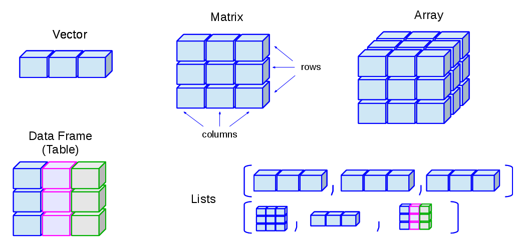
Data Stucture in R (ref: First Steps in R)
Interactive Matrix
Matrix Topics
viewof distTypeMat = Inputs.radio(
[
"Create / Inspect",
"Bind rows & cols (rbind/cbind)",
"Indexing [i, j] & slices",
"Assign / Replace (with NA)",
"Row/Col sums & means (apply)",
"Element-wise vs %*%",
"Transpose / diag() / Identity",
"Determinant & Inverse",
"Solve Ax = b",
"Eigen / SVD / Rank",
"Reshape & Vectorize",
"Kronecker ⊗ & outer()",
"Heatmap (no clustering)"
],
{ label: "", value: "Create / Inspect", inline: true }
)
Matrix
In R, matrices are two-dimensional, rectangular data structures.
They can only contain elements of a single data type (e.g., all numeric, all character, etc.).
How the create the matrix
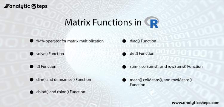
Create a matrix object using the matrix() function.
\[mat.A = \begin{bmatrix} 1&2&3&4\end{bmatrix}\]
\[mat.B = \begin{bmatrix} 1\\2\\3\\4\end{bmatrix}\]
\[mat.C = \begin{bmatrix} 1&3\\2&4\end{bmatrix}\]
\[mat.D = \begin{bmatrix} 1&2\\3&4\end{bmatrix}\]
The matrix in R is not the same as the matrix in linear algebra because of the multiplication and division operations.
\[mat.C\times mat.D = \begin{bmatrix} 1&3\\2&4\end{bmatrix} \times \begin{bmatrix} 1&2\\3&4\end{bmatrix}=\begin{bmatrix} 10&14\\14&20\end{bmatrix}\]
The multiplication operation uses the %*% function
Matrix transpose
We can compute the matrix transpose using the t() function
\[mat.A^T = \begin{bmatrix} 1&2&3&4\end{bmatrix}^T=\begin{bmatrix} 1\\2\\3\\4\end{bmatrix}\]
\[mat.B^T = \begin{bmatrix} 1\\2\\3\\4\end{bmatrix}^T=\begin{bmatrix} 1&2&3&4\end{bmatrix}\]
\[mat.C^T = \begin{bmatrix} 1&3\\2&4\end{bmatrix}^T=\begin{bmatrix} 1&2\\3&4\end{bmatrix}\]
\[mat.D^T = \begin{bmatrix} 1&2\\3&4\end{bmatrix}^T=\begin{bmatrix} 1&3\\2&4\end{bmatrix}\]
Matrix determinant
We use the det() function. (For square matrix only)
\[\begin{aligned} det(mat.C) &= det\left(\begin{bmatrix} 1&3\\2&4\end{bmatrix}\right)\\&=(1\times 4)-(2\times 3) \\&= -2\end{aligned}\]
\[\begin{aligned}det(mat.D) &= det\left(\begin{bmatrix} 1&2\\3&4\end{bmatrix}\right)\\&=(1\times 4)-(3\times 2) \\&= -2 \end{aligned}\]
Matrix inverse
We use the solve() function. (For square matrix only)
\[\begin{aligned}mat.C^{-1}&=\dfrac{1}{det(mat.C)}\begin{bmatrix} 4&-3\\-2&1\end{bmatrix}\\&=\dfrac{1}{-2}\begin{bmatrix} 4&-3\\-2&1\end{bmatrix}\\&=\begin{bmatrix} -2&1.5\\1&-0.5\end{bmatrix}\end{aligned}\]
\[\begin{aligned}mat.D^{-1}&=\dfrac{1}{det(mat.D)}\begin{bmatrix} 4&-2\\-3&1\end{bmatrix}\\&=\dfrac{1}{-2}\begin{bmatrix} 4&-3\\-2&1\end{bmatrix}\\&=\begin{bmatrix} -2&1\\1.5&-0.5\end{bmatrix}\end{aligned}\]
Solve the linear equation system \(Ax=B\)
Let
\[A=\begin{bmatrix}1&3\\2&4\end{bmatrix},~x=\begin{bmatrix}x_1\\x_2\end{bmatrix},~B=\begin{bmatrix}5\\13\end{bmatrix} \]
We can solve the linear equation system with the solve() function too. \[\begin{align*}
Ax&=B\\
\begin{bmatrix}1&3\\2&4\end{bmatrix}\begin{bmatrix} x_1\\x_2\end{bmatrix}&=\begin{bmatrix} 5\\13\end{bmatrix}
\end{align*}\]
How to access/edit the matrix
\[mat.E = \begin{bmatrix} 1&2&3\\4&5&6\\7&8&9\end{bmatrix}\]
1. Access a specific element
To access the element at row 2, column 2 of a matrix mat.E
2. Access an entire row
To access the entire second row of mat.E
or
or
3. Access an entire column
To access the entire third column of mat.E
4. Access a submatrix
You can also create a submatrix by specifying the row and column indices. For example, to extract a 2x2 submatrix from mat.E
From the object mat.E, show the values in rows 1 and 3 only.
Don’t show row 2
From the object mat.E, show the values in rows 3 and 1 respectively.
Don’t show row 2 and col 2
or
6. Access using logical conditions
To access elements that satisfy a certain condition, for example, elements greater than 5
7. Assign values to specific elements
You can also assign new values to specific elements in the matrix. For example:
Assign the previous value to a object mat.E.
change the value inside matrix
change the mat.F at (1,1) and (2,2) to 5
or use the diag() function. (diag = diagonal)
From the object mat.F, change the values in the first row to 1 and 2 respectively.
Merging two matrices with the cbind() and rbind() functions.
\[A=\begin{bmatrix}1&3\\2&4\end{bmatrix}\]
\[B=\begin{bmatrix}5&7\\6&8\end{bmatrix}\]
cbind() function: Merge by column
\[\begin{bmatrix}A&B\end{bmatrix}=\begin{bmatrix}1&3&5&7\\2&4&6&8\end{bmatrix}\]
\[\begin{bmatrix}B&A\end{bmatrix}=\begin{bmatrix}5&7&1&3\\6&8&2&4\end{bmatrix}\]
rbind() function: Merge by row
\[\begin{bmatrix}A\\B\end{bmatrix}=\begin{bmatrix}1&3\\2&4\\5&7\\6&8\end{bmatrix}\]
\[\begin{bmatrix}B\\A\end{bmatrix}=\begin{bmatrix}5&7\\6&8\\1&3\\2&4\end{bmatrix}\]
Exercise: Matrix Part 1
Exercise 1: Create a Matrix
Create a 3 × 3 matrix with the numbers 1 to 9, filled by rows.
Target output
     [,1] [,2] [,3]
[1,]    1    2    3
[2,]    4    5    6
[3,]    7    8    9
Complete the code
my_matrix <- (, nrow = , byrow = )
my_matrix
my_matrix
Hint: Use matrix() to create a matrix. Use numbers 1 to 9, set nrow = 3, and byrow = TRUE.
viewof var_ex1_create_matrix_1 = html`<input type="text" class="ojs-hidden-ex1_create_matrix" data-ojs-proxy="ex1_create_matrix::var_ex1_create_matrix_1" value="">`
viewof var_ex1_create_matrix_2 = html`<input type="text" class="ojs-hidden-ex1_create_matrix" data-ojs-proxy="ex1_create_matrix::var_ex1_create_matrix_2" value="">`
viewof var_ex1_create_matrix_3 = html`<input type="text" class="ojs-hidden-ex1_create_matrix" data-ojs-proxy="ex1_create_matrix::var_ex1_create_matrix_3" value="">`
viewof var_ex1_create_matrix_4 = html`<input type="text" class="ojs-hidden-ex1_create_matrix" data-ojs-proxy="ex1_create_matrix::var_ex1_create_matrix_4" value="">`
viewof var_ex1_create_matrix_run = html`<input type="number" class="ojs-hidden-ex1_create_matrix" data-ojs-run="ex1_create_matrix" value="0">`
Exercise 2: Access Matrix Elements
Access the element in the second row and third column of my_matrix.
Target output
[1] 6Complete the code
my_matrix <- matrix(1:9, nrow = 3, byrow = TRUE)
element <- [, ]
element
element <- [, ]
element
Hint: Use square brackets [] to access matrix elements. The format is matrix_name[row, column].
viewof var_ex2_access_matrix_1 = html`<input type="text" class="ojs-hidden-ex2_access_matrix" data-ojs-proxy="ex2_access_matrix::var_ex2_access_matrix_1" value="">`
viewof var_ex2_access_matrix_2 = html`<input type="text" class="ojs-hidden-ex2_access_matrix" data-ojs-proxy="ex2_access_matrix::var_ex2_access_matrix_2" value="">`
viewof var_ex2_access_matrix_3 = html`<input type="text" class="ojs-hidden-ex2_access_matrix" data-ojs-proxy="ex2_access_matrix::var_ex2_access_matrix_3" value="">`
viewof var_ex2_access_matrix_run = html`<input type="number" class="ojs-hidden-ex2_access_matrix" data-ojs-run="ex2_access_matrix" value="0">`
Exercise 3: Matrix Dimensions
Find the number of rows and columns in my_matrix. Hint: use dim() function.
Target output
[1] 3 3Complete the code
my_matrix <- matrix(1:9, nrow = 3, byrow = TRUE)
dims <- ()
dims
dims <- ()
dims
Hint: Use dim() to find matrix dimensions. It returns the number of rows and columns.
viewof var_ex3_matrix_dimensions_1 = html`<input type="text" class="ojs-hidden-ex3_matrix_dimensions" data-ojs-proxy="ex3_matrix_dimensions::var_ex3_matrix_dimensions_1" value="">`
viewof var_ex3_matrix_dimensions_2 = html`<input type="text" class="ojs-hidden-ex3_matrix_dimensions" data-ojs-proxy="ex3_matrix_dimensions::var_ex3_matrix_dimensions_2" value="">`
viewof var_ex3_matrix_dimensions_run = html`<input type="number" class="ojs-hidden-ex3_matrix_dimensions" data-ojs-run="ex3_matrix_dimensions" value="0">`
Exercise 4: Matrix Addition
Create another 3 × 3 matrix my_matrix2 with values 9 to 1 filled by rows. Then add my_matrix and my_matrix2 together.
Target output
     [,1] [,2] [,3]
[1,]   10   10   10
[2,]   10   10   10
[3,]   10   10   10
Complete the code
my_matrix <- matrix(1:9, nrow = 3, byrow = TRUE)
my_matrix2 <- (, nrow = 3, byrow = TRUE)
result_matrix <- +
result_matrix
my_matrix2 <- (, nrow = 3, byrow = TRUE)
result_matrix <- +
result_matrix
Hint: Use matrix() to create my_matrix2. Then use + to add two matrices element by element.
viewof var_ex4_matrix_addition_1 = html`<input type="text" class="ojs-hidden-ex4_matrix_addition" data-ojs-proxy="ex4_matrix_addition::var_ex4_matrix_addition_1" value="">`
viewof var_ex4_matrix_addition_2 = html`<input type="text" class="ojs-hidden-ex4_matrix_addition" data-ojs-proxy="ex4_matrix_addition::var_ex4_matrix_addition_2" value="">`
viewof var_ex4_matrix_addition_3 = html`<input type="text" class="ojs-hidden-ex4_matrix_addition" data-ojs-proxy="ex4_matrix_addition::var_ex4_matrix_addition_3" value="">`
viewof var_ex4_matrix_addition_4 = html`<input type="text" class="ojs-hidden-ex4_matrix_addition" data-ojs-proxy="ex4_matrix_addition::var_ex4_matrix_addition_4" value="">`
viewof var_ex4_matrix_addition_run = html`<input type="number" class="ojs-hidden-ex4_matrix_addition" data-ojs-run="ex4_matrix_addition" value="0">`
Exercise 5: Matrix Multiplication
Perform matrix multiplication between my_matrix and my_matrix2.
Target output
     [,1] [,2] [,3]
[1,]   30   24   18
[2,]   84   69   54
[3,]  138  114   90
Complete the code
my_matrix <- matrix(1:9, nrow = 3, byrow = TRUE)
my_matrix2 <- matrix(9:1, nrow = 3, byrow = TRUE)
product_matrix <-
product_matrix
my_matrix2 <- matrix(9:1, nrow = 3, byrow = TRUE)
product_matrix <-
product_matrix
Hint: Use %*% for matrix multiplication in R. Do not use * or +.
viewof var_ex5_matrix_multiplication_1 = html`<input type="text" class="ojs-hidden-ex5_matrix_multiplication" data-ojs-proxy="ex5_matrix_multiplication::var_ex5_matrix_multiplication_1" value="">`
viewof var_ex5_matrix_multiplication_2 = html`<input type="text" class="ojs-hidden-ex5_matrix_multiplication" data-ojs-proxy="ex5_matrix_multiplication::var_ex5_matrix_multiplication_2" value="">`
viewof var_ex5_matrix_multiplication_3 = html`<input type="text" class="ojs-hidden-ex5_matrix_multiplication" data-ojs-proxy="ex5_matrix_multiplication::var_ex5_matrix_multiplication_3" value="">`
viewof var_ex5_matrix_multiplication_run = html`<input type="number" class="ojs-hidden-ex5_matrix_multiplication" data-ojs-run="ex5_matrix_multiplication" value="0">`
Exercise 6: Transpose a Matrix
Find the transpose of my_matrix.
Target output
     [,1] [,2] [,3]
[1,]    1    4    7
[2,]    2    5    8
[3,]    3    6    9
Complete the code
my_matrix <- matrix(1:9, nrow = 3, byrow = TRUE)
transposed_matrix <- ()
transposed_matrix
transposed_matrix <- ()
transposed_matrix
Hint: Use t() to transpose a matrix. It swaps rows and columns.
viewof var_ex6_transpose_matrix_1 = html`<input type="text" class="ojs-hidden-ex6_transpose_matrix" data-ojs-proxy="ex6_transpose_matrix::var_ex6_transpose_matrix_1" value="">`
viewof var_ex6_transpose_matrix_2 = html`<input type="text" class="ojs-hidden-ex6_transpose_matrix" data-ojs-proxy="ex6_transpose_matrix::var_ex6_transpose_matrix_2" value="">`
viewof var_ex6_transpose_matrix_run = html`<input type="number" class="ojs-hidden-ex6_transpose_matrix" data-ojs-run="ex6_transpose_matrix" value="0">`
Exercise 7: Matrix Determinant
Calculate the determinant of a 2 × 2 matrix my_matrix3 with values 4, 7, 2, and 6.
Target output
[1] 10Complete the code
my_matrix3 <- (, nrow = 2)
det_value <- ()
det_value
det_value <- ()
det_value
Hint: Use matrix() to create a 2×2 matrix and det() to calculate its determinant.
viewof var_ex7_matrix_determinant_1 = html`<input type="text" class="ojs-hidden-ex7_matrix_determinant" data-ojs-proxy="ex7_matrix_determinant::var_ex7_matrix_determinant_1" value="">`
viewof var_ex7_matrix_determinant_2 = html`<input type="text" class="ojs-hidden-ex7_matrix_determinant" data-ojs-proxy="ex7_matrix_determinant::var_ex7_matrix_determinant_2" value="">`
viewof var_ex7_matrix_determinant_3 = html`<input type="text" class="ojs-hidden-ex7_matrix_determinant" data-ojs-proxy="ex7_matrix_determinant::var_ex7_matrix_determinant_3" value="">`
viewof var_ex7_matrix_determinant_4 = html`<input type="text" class="ojs-hidden-ex7_matrix_determinant" data-ojs-proxy="ex7_matrix_determinant::var_ex7_matrix_determinant_4" value="">`
viewof var_ex7_matrix_determinant_run = html`<input type="number" class="ojs-hidden-ex7_matrix_determinant" data-ojs-run="ex7_matrix_determinant" value="0">`
Exercise 8: Inverse of a Matrix
Find the inverse of my_matrix3, if it exists.
Target output
     [,1] [,2]
[1,]  0.6 -0.2
[2,] -0.7  0.4
Complete the code
my_matrix3 <- matrix(c(4, 7, 2, 6), nrow = 2)
inverse_matrix <- ()
inverse_matrix
inverse_matrix <- ()
inverse_matrix
Hint: Use solve() to calculate the inverse of a matrix. The matrix must be invertible.
viewof var_ex8_inverse_matrix_1 = html`<input type="text" class="ojs-hidden-ex8_inverse_matrix" data-ojs-proxy="ex8_inverse_matrix::var_ex8_inverse_matrix_1" value="">`
viewof var_ex8_inverse_matrix_2 = html`<input type="text" class="ojs-hidden-ex8_inverse_matrix" data-ojs-proxy="ex8_inverse_matrix::var_ex8_inverse_matrix_2" value="">`
viewof var_ex8_inverse_matrix_run = html`<input type="number" class="ojs-hidden-ex8_inverse_matrix" data-ojs-run="ex8_inverse_matrix" value="0">`
Exercise 9: Diagonal of a Matrix
Extract the diagonal elements of my_matrix.
Target output
[1] 1 5 9Complete the code
my_matrix <- matrix(1:9, nrow = 3, byrow = TRUE)
diagonal_elements <- ()
diagonal_elements
diagonal_elements <- ()
diagonal_elements
Hint: Use diag() to extract diagonal elements from a matrix.
viewof var_ex9_matrix_diagonal_1 = html`<input type="text" class="ojs-hidden-ex9_matrix_diagonal" data-ojs-proxy="ex9_matrix_diagonal::var_ex9_matrix_diagonal_1" value="">`
viewof var_ex9_matrix_diagonal_2 = html`<input type="text" class="ojs-hidden-ex9_matrix_diagonal" data-ojs-proxy="ex9_matrix_diagonal::var_ex9_matrix_diagonal_2" value="">`
viewof var_ex9_matrix_diagonal_run = html`<input type="number" class="ojs-hidden-ex9_matrix_diagonal" data-ojs-run="ex9_matrix_diagonal" value="0">`
Exercise 10: Create an Identity Matrix
Create a 4 × 4 identity matrix.
Target output
     [,1] [,2] [,3] [,4]
[1,]    1    0    0    0
[2,]    0    1    0    0
[3,]    0    0    1    0
[4,]    0    0    0    1
Complete the code
identity_matrix <- ()
identity_matrix
identity_matrix
Hint: Use diag(n) to create an n × n identity matrix.
viewof var_ex10_identity_matrix_1 = html`<input type="text" class="ojs-hidden-ex10_identity_matrix" data-ojs-proxy="ex10_identity_matrix::var_ex10_identity_matrix_1" value="">`
viewof var_ex10_identity_matrix_2 = html`<input type="text" class="ojs-hidden-ex10_identity_matrix" data-ojs-proxy="ex10_identity_matrix::var_ex10_identity_matrix_2" value="">`
viewof var_ex10_identity_matrix_run = html`<input type="number" class="ojs-hidden-ex10_identity_matrix" data-ojs-run="ex10_identity_matrix" value="0">`
Exercise: Matrix part 2
The exercises 11 to 20 focusing on data manipulation with matrix objects in R:
Exercise 11: Element-wise Multiplication
Perform element-wise multiplication between my_matrix and a matrix of the same dimensions containing all 2’s.
Target output
     [,1] [,2] [,3]
[1,]    2    4    6
[2,]    8   10   12
[3,]   14   16   18
Complete the code
my_matrix <- matrix(1:9, nrow = 3, byrow = TRUE)
result_matrix <- (, nrow = 3, ncol = 3)
result_matrix
result_matrix <- (, nrow = 3, ncol = 3)
result_matrix
Hint: Use * for element-wise multiplication and matrix() to create a 3 × 3 matrix filled with 2's.
viewof var_ex11_elementwise_multiplication_1 = html`<input type="text" class="ojs-hidden-ex11_elementwise_multiplication" data-ojs-proxy="ex11_elementwise_multiplication::var_ex11_elementwise_multiplication_1" value="">`
viewof var_ex11_elementwise_multiplication_2 = html`<input type="text" class="ojs-hidden-ex11_elementwise_multiplication" data-ojs-proxy="ex11_elementwise_multiplication::var_ex11_elementwise_multiplication_2" value="">`
viewof var_ex11_elementwise_multiplication_3 = html`<input type="text" class="ojs-hidden-ex11_elementwise_multiplication" data-ojs-proxy="ex11_elementwise_multiplication::var_ex11_elementwise_multiplication_3" value="">`
viewof var_ex11_elementwise_multiplication_4 = html`<input type="text" class="ojs-hidden-ex11_elementwise_multiplication" data-ojs-proxy="ex11_elementwise_multiplication::var_ex11_elementwise_multiplication_4" value="">`
viewof var_ex11_elementwise_multiplication_run = html`<input type="number" class="ojs-hidden-ex11_elementwise_multiplication" data-ojs-run="ex11_elementwise_multiplication" value="0">`
Exercise 12: Row and Column Sums
Calculate the sum of each row and each column in my_matrix.
Target output
[1] 6 15 24[1] 12 15 18Complete the code
my_matrix <- matrix(1:9, nrow = 3, byrow = TRUE)
row_sums <- ()
col_sums <- ()
row_sums
col_sums
row_sums <- ()
col_sums <- ()
row_sums
col_sums
Hint: Use rowSums() to sum each row and colSums() to sum each column.
viewof var_ex12_row_col_sums_1 = html`<input type="text" class="ojs-hidden-ex12_row_col_sums" data-ojs-proxy="ex12_row_col_sums::var_ex12_row_col_sums_1" value="">`
viewof var_ex12_row_col_sums_2 = html`<input type="text" class="ojs-hidden-ex12_row_col_sums" data-ojs-proxy="ex12_row_col_sums::var_ex12_row_col_sums_2" value="">`
viewof var_ex12_row_col_sums_3 = html`<input type="text" class="ojs-hidden-ex12_row_col_sums" data-ojs-proxy="ex12_row_col_sums::var_ex12_row_col_sums_3" value="">`
viewof var_ex12_row_col_sums_4 = html`<input type="text" class="ojs-hidden-ex12_row_col_sums" data-ojs-proxy="ex12_row_col_sums::var_ex12_row_col_sums_4" value="">`
viewof var_ex12_row_col_sums_run = html`<input type="number" class="ojs-hidden-ex12_row_col_sums" data-ojs-run="ex12_row_col_sums" value="0">`
Exercise 13: Add a Row to a Matrix
Add a new row c(10, 11, 12) to my_matrix and create my_matrix_extended.
Target output
        [,1] [,2] [,3]
           1    2    3
           4    5    6
           7    8    9
new_row   10   11   12
Complete the code
my_matrix <- matrix(1:9, nrow = 3, byrow = TRUE)
new_row <- ()
my_matrix_extended <- (, )
my_matrix_extended
new_row <- ()
my_matrix_extended <- (, )
my_matrix_extended
Hint: Use c() to create the new row and rbind() to add a row to a matrix.
viewof var_ex13_add_row_matrix_1 = html`<input type="text" class="ojs-hidden-ex13_add_row_matrix" data-ojs-proxy="ex13_add_row_matrix::var_ex13_add_row_matrix_1" value="">`
viewof var_ex13_add_row_matrix_2 = html`<input type="text" class="ojs-hidden-ex13_add_row_matrix" data-ojs-proxy="ex13_add_row_matrix::var_ex13_add_row_matrix_2" value="">`
viewof var_ex13_add_row_matrix_3 = html`<input type="text" class="ojs-hidden-ex13_add_row_matrix" data-ojs-proxy="ex13_add_row_matrix::var_ex13_add_row_matrix_3" value="">`
viewof var_ex13_add_row_matrix_4 = html`<input type="text" class="ojs-hidden-ex13_add_row_matrix" data-ojs-proxy="ex13_add_row_matrix::var_ex13_add_row_matrix_4" value="">`
viewof var_ex13_add_row_matrix_5 = html`<input type="text" class="ojs-hidden-ex13_add_row_matrix" data-ojs-proxy="ex13_add_row_matrix::var_ex13_add_row_matrix_5" value="">`
viewof var_ex13_add_row_matrix_run = html`<input type="number" class="ojs-hidden-ex13_add_row_matrix" data-ojs-run="ex13_add_row_matrix" value="0">`
Exercise 14: Add a Column to a Matrix
Add a new column c(13, 14, 15, 16) to my_matrix_extended.
Target output
                 new_column
         1  2  3         13
         4  5  6         14
         7  8  9         15
new_row 10 11 12         16
Complete the code
my_matrix <- matrix(1:9, nrow = 3, byrow = TRUE)
new_row <- c(10, 11, 12)
my_matrix_extended <- rbind(my_matrix, new_row)
new_column <- ()
my_matrix_extended <- (, )
my_matrix_extended
new_row <- c(10, 11, 12)
my_matrix_extended <- rbind(my_matrix, new_row)
new_column <- ()
my_matrix_extended <- (, )
my_matrix_extended
Hint: Use c() to create the new column and cbind() to add a column to a matrix.
viewof var_ex14_add_column_matrix_1 = html`<input type="text" class="ojs-hidden-ex14_add_column_matrix" data-ojs-proxy="ex14_add_column_matrix::var_ex14_add_column_matrix_1" value="">`
viewof var_ex14_add_column_matrix_2 = html`<input type="text" class="ojs-hidden-ex14_add_column_matrix" data-ojs-proxy="ex14_add_column_matrix::var_ex14_add_column_matrix_2" value="">`
viewof var_ex14_add_column_matrix_3 = html`<input type="text" class="ojs-hidden-ex14_add_column_matrix" data-ojs-proxy="ex14_add_column_matrix::var_ex14_add_column_matrix_3" value="">`
viewof var_ex14_add_column_matrix_4 = html`<input type="text" class="ojs-hidden-ex14_add_column_matrix" data-ojs-proxy="ex14_add_column_matrix::var_ex14_add_column_matrix_4" value="">`
viewof var_ex14_add_column_matrix_5 = html`<input type="text" class="ojs-hidden-ex14_add_column_matrix" data-ojs-proxy="ex14_add_column_matrix::var_ex14_add_column_matrix_5" value="">`
viewof var_ex14_add_column_matrix_run = html`<input type="number" class="ojs-hidden-ex14_add_column_matrix" data-ojs-run="ex14_add_column_matrix" value="0">`
Exercise 15: Subsetting a Matrix
Extract a submatrix from my_matrix that includes the first two rows and the last two columns.
Target output
     [,1] [,2]
[1,]    2    3
[2,]    5    6
Complete the code
my_matrix <- matrix(1:9, nrow = 3, byrow = TRUE)
sub_matrix <- [, ]
sub_matrix
sub_matrix <- [, ]
sub_matrix
Hint: Use matrix[row_range, column_range]. The first two rows are 1:2 and the last two columns are 2:3.
viewof var_ex15_subsetting_matrix_1 = html`<input type="text" class="ojs-hidden-ex15_subsetting_matrix" data-ojs-proxy="ex15_subsetting_matrix::var_ex15_subsetting_matrix_1" value="">`
viewof var_ex15_subsetting_matrix_2 = html`<input type="text" class="ojs-hidden-ex15_subsetting_matrix" data-ojs-proxy="ex15_subsetting_matrix::var_ex15_subsetting_matrix_2" value="">`
viewof var_ex15_subsetting_matrix_3 = html`<input type="text" class="ojs-hidden-ex15_subsetting_matrix" data-ojs-proxy="ex15_subsetting_matrix::var_ex15_subsetting_matrix_3" value="">`
viewof var_ex15_subsetting_matrix_run = html`<input type="number" class="ojs-hidden-ex15_subsetting_matrix" data-ojs-run="ex15_subsetting_matrix" value="0">`
Exercise 16: Replace Elements in a Matrix
Replace all elements in my_matrix that are greater than 5 with the value 0.
Target output
     [,1] [,2] [,3]
[1,]    1    2    3
[2,]    4    5    0
[3,]    0    0    0
Complete the code
my_matrix <- matrix(1:9, nrow = 3, byrow = TRUE)
[ > ] <-
my_matrix
[ > ] <-
my_matrix
Hint: Use logical indexing: matrix[matrix > value] <- new_value
viewof var_ex16_replace_elements_matrix_1 = html`<input type="text" class="ojs-hidden-ex16_replace_elements_matrix" data-ojs-proxy="ex16_replace_elements_matrix::var_ex16_replace_elements_matrix_1" value="">`
viewof var_ex16_replace_elements_matrix_2 = html`<input type="text" class="ojs-hidden-ex16_replace_elements_matrix" data-ojs-proxy="ex16_replace_elements_matrix::var_ex16_replace_elements_matrix_2" value="">`
viewof var_ex16_replace_elements_matrix_3 = html`<input type="text" class="ojs-hidden-ex16_replace_elements_matrix" data-ojs-proxy="ex16_replace_elements_matrix::var_ex16_replace_elements_matrix_3" value="">`
viewof var_ex16_replace_elements_matrix_4 = html`<input type="text" class="ojs-hidden-ex16_replace_elements_matrix" data-ojs-proxy="ex16_replace_elements_matrix::var_ex16_replace_elements_matrix_4" value="">`
viewof var_ex16_replace_elements_matrix_run = html`<input type="number" class="ojs-hidden-ex16_replace_elements_matrix" data-ojs-run="ex16_replace_elements_matrix" value="0">`
Exercise 17: Matrix Mean
Calculate the mean of all the elements in my_matrix.
Target output
[1] 5Complete the code
my_matrix <- matrix(1:9, nrow = 3, byrow = TRUE)
matrix_mean <- ()
matrix_mean
matrix_mean <- ()
matrix_mean
Hint: Use mean() to calculate the average of all elements in a matrix.
viewof var_ex17_matrix_mean_1 = html`<input type="text" class="ojs-hidden-ex17_matrix_mean" data-ojs-proxy="ex17_matrix_mean::var_ex17_matrix_mean_1" value="">`
viewof var_ex17_matrix_mean_2 = html`<input type="text" class="ojs-hidden-ex17_matrix_mean" data-ojs-proxy="ex17_matrix_mean::var_ex17_matrix_mean_2" value="">`
viewof var_ex17_matrix_mean_run = html`<input type="number" class="ojs-hidden-ex17_matrix_mean" data-ojs-run="ex17_matrix_mean" value="0">`
Exercise 18: Apply a Function to Rows or Columns
Use the apply() function to calculate the product of each row in my_matrix.
Target output
[1] 6 120 504Complete the code
my_matrix <- matrix(1:9, nrow = 3, byrow = TRUE)
row_products <- (, , )
row_products
row_products <- (, , )
row_products
Hint: Use apply(X, MARGIN, FUN). MARGIN = 1 means rows, and prod calculates product.
viewof var_ex18_apply_function_1 = html`<input type="text" class="ojs-hidden-ex18_apply_function" data-ojs-proxy="ex18_apply_function::var_ex18_apply_function_1" value="">`
viewof var_ex18_apply_function_2 = html`<input type="text" class="ojs-hidden-ex18_apply_function" data-ojs-proxy="ex18_apply_function::var_ex18_apply_function_2" value="">`
viewof var_ex18_apply_function_3 = html`<input type="text" class="ojs-hidden-ex18_apply_function" data-ojs-proxy="ex18_apply_function::var_ex18_apply_function_3" value="">`
viewof var_ex18_apply_function_4 = html`<input type="text" class="ojs-hidden-ex18_apply_function" data-ojs-proxy="ex18_apply_function::var_ex18_apply_function_4" value="">`
viewof var_ex18_apply_function_run = html`<input type="number" class="ojs-hidden-ex18_apply_function" data-ojs-run="ex18_apply_function" value="0">`
Exercise 19: Matrix to Vector
Convert my_matrix into a vector.
Target output
[1] 1 4 7 2 5 8 3 6 9Complete the code
my_matrix <- matrix(1:9, nrow = 3, byrow = TRUE)
matrix_vector <- ()
matrix_vector
matrix_vector <- ()
matrix_vector
Hint: Use as.vector() to convert a matrix into a vector.
viewof var_ex19_matrix_to_vector_1 = html`<input type="text" class="ojs-hidden-ex19_matrix_to_vector" data-ojs-proxy="ex19_matrix_to_vector::var_ex19_matrix_to_vector_1" value="">`
viewof var_ex19_matrix_to_vector_2 = html`<input type="text" class="ojs-hidden-ex19_matrix_to_vector" data-ojs-proxy="ex19_matrix_to_vector::var_ex19_matrix_to_vector_2" value="">`
viewof var_ex19_matrix_to_vector_run = html`<input type="number" class="ojs-hidden-ex19_matrix_to_vector" data-ojs-run="ex19_matrix_to_vector" value="0">`
Exercise 20: Reshape a Matrix
Reshape my_matrix into a 1 × 9 matrix.
Target output
     [,1] [,2] [,3] [,4] [,5] [,6] [,7] [,8] [,9]
[1,]    1    4    7    2    5    8    3    6    9
Complete the code
my_matrix <- matrix(1:9, nrow = 3, byrow = TRUE)
reshaped_matrix <- (, nrow = )
reshaped_matrix
reshaped_matrix <- (, nrow = )
reshaped_matrix
Hint: Use matrix(data, nrow = ...) to reshape a matrix.
viewof var_ex20_reshape_matrix_1 = html`<input type="text" class="ojs-hidden-ex20_reshape_matrix" data-ojs-proxy="ex20_reshape_matrix::var_ex20_reshape_matrix_1" value="">`
viewof var_ex20_reshape_matrix_2 = html`<input type="text" class="ojs-hidden-ex20_reshape_matrix" data-ojs-proxy="ex20_reshape_matrix::var_ex20_reshape_matrix_2" value="">`
viewof var_ex20_reshape_matrix_3 = html`<input type="text" class="ojs-hidden-ex20_reshape_matrix" data-ojs-proxy="ex20_reshape_matrix::var_ex20_reshape_matrix_3" value="">`
viewof var_ex20_reshape_matrix_run = html`<input type="number" class="ojs-hidden-ex20_reshape_matrix" data-ojs-run="ex20_reshape_matrix" value="0">`
Exercise 21: Matrix Subtraction
Subtract my_matrix2 from my_matrix.
Target output
     [,1] [,2] [,3]
[1,]   -8   -6   -4
[2,]   -2    0    2
[3,]    4    6    8
Complete the code
result_matrix <-
result_matrix
result_matrix
Hint: Use - for matrix subtraction.
viewof var_ex21_matrix_subtraction_1 = html`<input type="text" class="ojs-hidden-ex21_matrix_subtraction" data-ojs-proxy="ex21_matrix_subtraction::var_ex21_matrix_subtraction_1" value="">`
viewof var_ex21_matrix_subtraction_2 = html`<input type="text" class="ojs-hidden-ex21_matrix_subtraction" data-ojs-proxy="ex21_matrix_subtraction::var_ex21_matrix_subtraction_2" value="">`
viewof var_ex21_matrix_subtraction_3 = html`<input type="text" class="ojs-hidden-ex21_matrix_subtraction" data-ojs-proxy="ex21_matrix_subtraction::var_ex21_matrix_subtraction_3" value="">`
viewof var_ex21_matrix_subtraction_run = html`<input type="number" class="ojs-hidden-ex21_matrix_subtraction" data-ojs-run="ex21_matrix_subtraction" value="0">`
Exercise 22: Matrix Trace
Calculate the trace of my_matrix.
Target output
[1] 15Complete the code
trace_value <- (())
trace_value
trace_value
Hint: Trace = sum of diagonal elements.
viewof var_ex22_matrix_trace_1 = html`<input type="text" class="ojs-hidden-ex22_matrix_trace" data-ojs-proxy="ex22_matrix_trace::var_ex22_matrix_trace_1" value="">`
viewof var_ex22_matrix_trace_2 = html`<input type="text" class="ojs-hidden-ex22_matrix_trace" data-ojs-proxy="ex22_matrix_trace::var_ex22_matrix_trace_2" value="">`
viewof var_ex22_matrix_trace_3 = html`<input type="text" class="ojs-hidden-ex22_matrix_trace" data-ojs-proxy="ex22_matrix_trace::var_ex22_matrix_trace_3" value="">`
viewof var_ex22_matrix_trace_run = html`<input type="number" class="ojs-hidden-ex22_matrix_trace" data-ojs-run="ex22_matrix_trace" value="0">`
Exercise 23: Maximum Value in Matrix
Find the maximum value in my_matrix.
Target output
[1] 9Complete the code
max_value <- ()
max_value
max_value
Hint: Use max().
viewof var_ex23_matrix_max_1 = html`<input type="text" class="ojs-hidden-ex23_matrix_max" data-ojs-proxy="ex23_matrix_max::var_ex23_matrix_max_1" value="">`
viewof var_ex23_matrix_max_2 = html`<input type="text" class="ojs-hidden-ex23_matrix_max" data-ojs-proxy="ex23_matrix_max::var_ex23_matrix_max_2" value="">`
viewof var_ex23_matrix_max_run = html`<input type="number" class="ojs-hidden-ex23_matrix_max" data-ojs-run="ex23_matrix_max" value="0">`
Exercise 24: Minimum Value in Matrix
Find the minimum value in my_matrix.
Target output
[1] 1Complete the code
min_value <- ()
min_value
min_value
Hint: Use min().
viewof var_ex24_matrix_min_1 = html`<input type="text" class="ojs-hidden-ex24_matrix_min" data-ojs-proxy="ex24_matrix_min::var_ex24_matrix_min_1" value="">`
viewof var_ex24_matrix_min_2 = html`<input type="text" class="ojs-hidden-ex24_matrix_min" data-ojs-proxy="ex24_matrix_min::var_ex24_matrix_min_2" value="">`
viewof var_ex24_matrix_min_run = html`<input type="number" class="ojs-hidden-ex24_matrix_min" data-ojs-run="ex24_matrix_min" value="0">`
Exercise 25: Matrix Standard Deviation
Calculate the standard deviation of all elements in my_matrix.
Target output
[1] 2.738613Complete the code
matrix_sd <- ()
matrix_sd
matrix_sd
Hint: Use sd() to calculate standard deviation.
viewof var_ex25_matrix_sd_1 = html`<input type="text" class="ojs-hidden-ex25_matrix_sd" data-ojs-proxy="ex25_matrix_sd::var_ex25_matrix_sd_1" value="">`
viewof var_ex25_matrix_sd_2 = html`<input type="text" class="ojs-hidden-ex25_matrix_sd" data-ojs-proxy="ex25_matrix_sd::var_ex25_matrix_sd_2" value="">`
viewof var_ex25_matrix_sd_run = html`<input type="number" class="ojs-hidden-ex25_matrix_sd" data-ojs-run="ex25_matrix_sd" value="0">`