margin → Add margins around text (margin(top, right, bottom, left))
Summary
Argument
Description
Example
family
Font family (e.g., "serif", "sans")
family = "serif"
face
Font style ("bold", "italic", etc.)
face = "bold"
size
Font size (in points)
size = 14
lineheight
Line spacing
lineheight = 1.5
color
Text color
color = "red"
alpha
Transparency (0 to 1)
alpha = 0.7
hjust
Horizontal justification (0 to 1)
hjust = 0.5
vjust
Vertical justification (0 to 1)
vjust = 1
angle
Rotate text (degrees)
angle = 45
margin
Margin around text
margin(5,5,5,5)
Summary of element_text() Usage in theme()
theme() Argument
Description
plot.title
Main title
plot.subtitle
Subtitle
plot.caption
Caption at bottom
plot.tag
Tag (e.g., “A”, “B”)
axis.title.x
X-axis title
axis.title.y
Y-axis title
axis.text.x
X-axis tick labels
axis.text.y
Y-axis tick labels
legend.title
Legend title
legend.text
Legend labels
strip.text.x
Facet labels (horizontal)
strip.text.y
Facet labels (vertical)
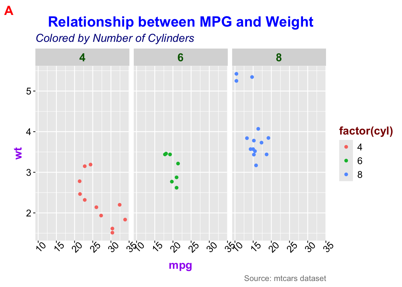
library(ggplot2)mtcars |>ggplot() +aes( x= mpg, y = wt, color =factor(cyl)) +geom_point() +facet_grid(.~cyl) +theme(# Plot title, subtitle, caption, and tagplot.title =element_text(size =18, face ="bold", color ="blue", hjust =0.5),plot.subtitle =element_text(size =14, face ="italic", color ="darkblue"),plot.caption =element_text(size =10, color ="gray50"),plot.tag =element_text(size =16, face ="bold", color ="red"),# Axis titlesaxis.title.x =element_text(size =14, face ="bold", color ="purple"),axis.title.y =element_text(size =14, face ="bold", color ="purple"),# Axis text (tick labels)axis.text.x =element_text(size =12, color ="black", angle =45, vjust =1),axis.text.y =element_text(size =12, color ="black"),# Legend title and textlegend.title =element_text(size =14, face ="bold", color ="darkred"),legend.text =element_text(size =12, color ="black"),# Facet strip textstrip.text.x =element_text(size =14, face ="bold", color ="darkgreen"),strip.text.y =element_text(size =14, face ="bold", color ="darkgreen") ) +labs(title ="Relationship between MPG and Weight",subtitle ="Colored by Number of Cylinders",caption ="Source: mtcars dataset",tag ="A" )
2. Background & Panel Elements
These control the background, grid, and panel appearance.
plot.background: Background of the entire plot.
panel.background: Background of the plotting area.
panel.grid: Grid lines.
panel.grid.major
panel.grid.minor
panel.border: Border around the plot panel.
panel.spacing: Spacing between facets.
3. Axis Customization
These control the appearance of axes and ticks.
axis.line: Axis lines.
axis.ticks: Ticks on the axes.
axis.ticks.x
axis.ticks.y
axis.text: Axis labels.
axis.text.x
axis.text.y
axis.title: Axis titles.
axis.title.x
axis.title.y
4. Legend Elements
These control the appearance of the legend.
legend.background: Background of the legend.
legend.key: Background of legend keys.
legend.key.size: Size of legend keys.
legend.position: Position of the legend.
"none", "left", "right", "top", "bottom"
legend.direction: Layout direction ("horizontal" or "vertical").
legend.box: Arrangement of multiple legends ("horizontal" or "vertical").
5. Facet Customization
These control the appearance of facet labels.
strip.background: Background color of facet labels.
strip.text: Text of facet labels.
strip.text.x
strip.text.y
strip.placement: Placement of facet labels ("inside" or "outside").
6. Margins & Spacing
These control spacing between different elements.
plot.margin: Margins around the plot.
legend.margin: Margins around the legend.
element_rect() function
The element_rect() function in ggplot2 is used within the theme() function to customize rectangular elements like backgrounds, borders, and legend keys.
The list of available arguments:
1. Fill & Border Color
fill → Background color (e.g., "red", "blue", "#123456", NA for transparent)
colour / color → Border color (same format as fill)
2. Border Line Settings
linewidth → Border line thickness (default 0.5)
linetype → Border line type:
1 or "solid" → Solid line
2 or "dashed" → Dashed line
3 or "dotted" → Dotted line
4 or "dotdash" → Dot-dash line
5 or "longdash" → Long dash
6 or "twodash" → Two dashes
3. Rounded Corners
r → Corner radius (default 0, set higher for rounded corners)
Summary of element_rect() Arguments
Argument
Description
Example
fill
Background color
fill = "gray90"
color / colour
Border color
colour = "black"
linewidth
Border thickness
linewidth = 1.5
linetype
Border line type
linetype = "dashed"
r
Corner radius (rounded corners)
r = 5
Summary of element_rect() Usage in theme()
theme() Argument
Description
plot.background
Entire plot background
panel.background
Plotting area background
panel.border
Border around the plotting area
legend.background
Background behind the legend
legend.box.background
Border around the legend box
legend.key
Background of legend keys
strip.background
Background of facet labels
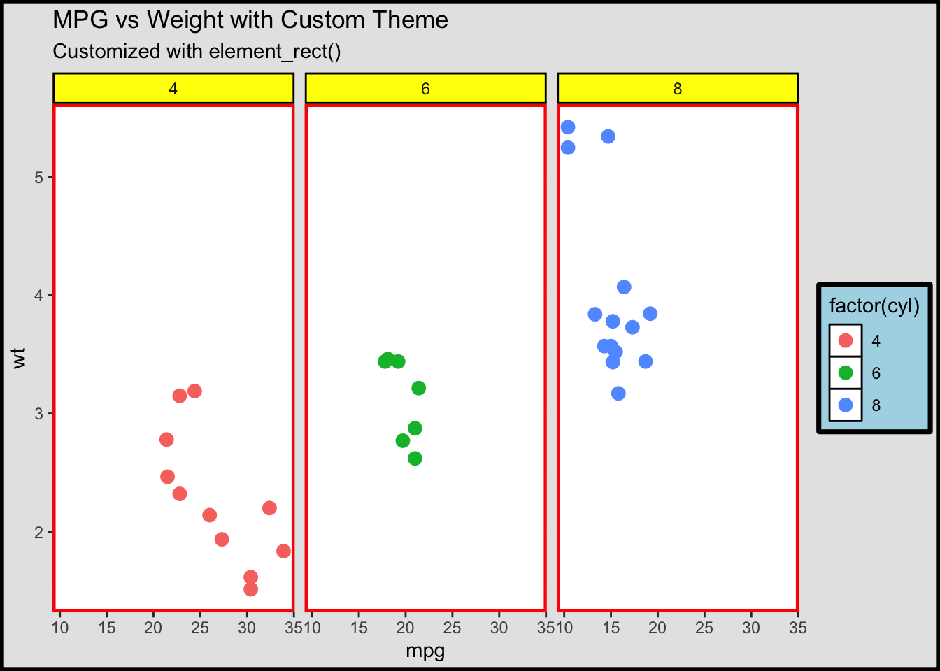
mtcars |>ggplot() +aes(x = mpg, y = wt, color =factor(cyl)) +geom_point(size =3) +facet_grid(.~cyl) +theme(# Background settingsplot.background =element_rect(fill ="gray90", color ="black", linewidth =2),panel.background =element_rect(fill ="white", color ="black", linewidth =1),# Borderspanel.border =element_rect(color ="red", fill =NA, linewidth =1.5),# Legendlegend.background =element_rect(fill ="lightblue", color ="black", linewidth =1),legend.box.background =element_rect(fill ="gray80", color ="black", linewidth =1.5),legend.key =element_rect(fill ="white", color ="black", linewidth =0.5),# Facet strip (for facet_wrap)strip.background =element_rect(fill ="yellow", color ="black", linewidth =1) ) +labs(title ="MPG vs Weight with Custom Theme",subtitle ="Customized with element_rect()" )
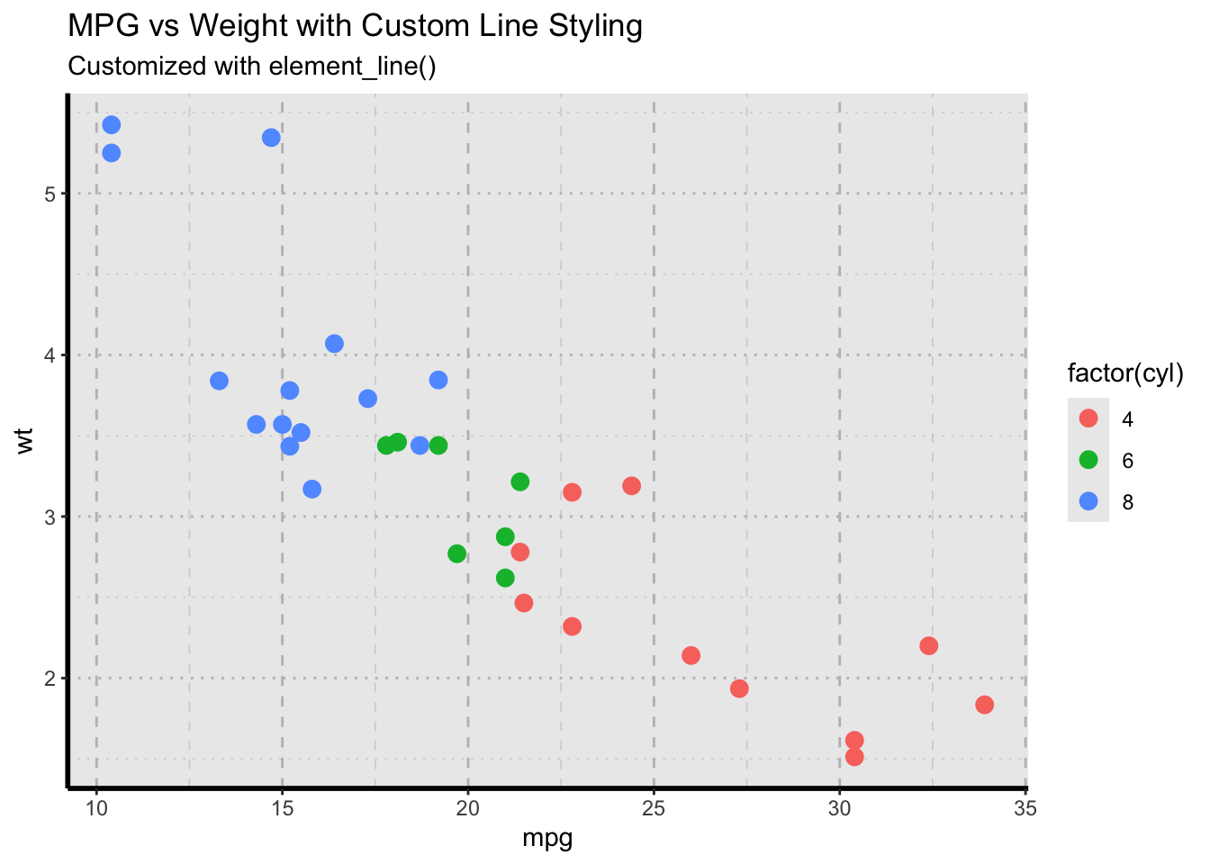
element_line() function
The element_line() function in ggplot2 is used within theme() to customize lines in a plot, such as axis lines, grid lines, and borders.
Arguments in element_line()
The list of available arguments:
1. Line Appearance
colour / color → Line color (e.g., "black", "red", "#123456")
The element_blank() function in ggplot2 is used within theme() to completely remove an element from a plot.
element_blank()removes an element completely.
Useful for minimalist plots.
Works inside theme() with axis labels, titles, grid lines, legends, backgrounds, etc..
Summary of element_blank() Usage in theme()
theme() Argument
Description
axis.text.x / axis.text.y
Remove axis text labels
axis.title.x / axis.title.y
Remove axis titles
axis.line.x / axis.line.y
Remove axis lines
axis.ticks.x / axis.ticks.y
Remove axis ticks
panel.grid.major / panel.grid.minor
Remove grid lines
plot.background
Remove the entire plot background
panel.background
Remove the background of the plotting area
panel.border
Remove the border around the plot panel
legend.background
Remove the legend background
legend.key
Remove the background of legend items
legend.title
Remove the legend title
legend.text
Remove the legend text
strip.background
Remove the background of facet labels
strip.text
Remove the text inside facet labels
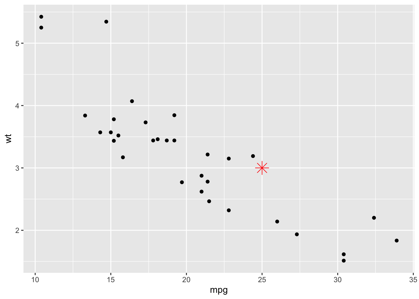
annotae() function
The annotate() function in ggplot2 allows you to add text, shapes, or other graphical elements to a plot. It is particularly useful for adding annotations that are not tied to data points but rather placed at specific coordinates.
Syntax of annotate()
annotate(geom, x, y, label =NULL, color ="black", size =5, ...)
geom → Type of annotation ("text", "label", "rect", "segment", "point", etc.).
x, y → Position coordinates for the annotation.
label → Text to be displayed (if geom = "text" or geom = "label").
color → Color of the annotation.
size → Size of text or shape.
Additional parameters depending on the geom.
Examples of annotate() Usage
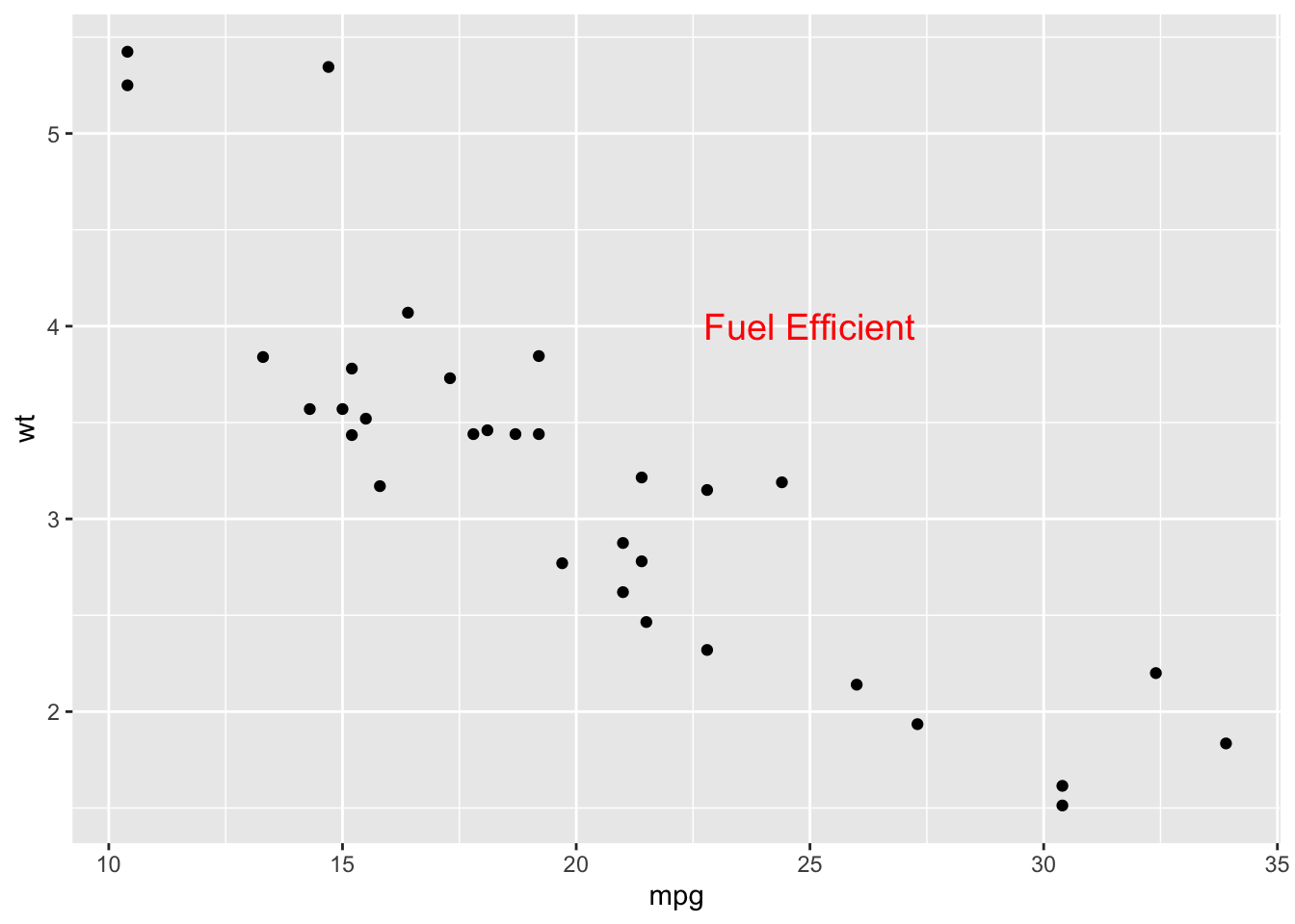
1️) Adding Text Annotation
library(ggplot2)mtcars |>ggplot() +aes(x = mpg, y = wt) +geom_point() +annotate(geom ="text", x =25, y =4, label ="Fuel Efficient", color ="red", size =5)
🔹 Adds a red text label at (x = 25, y = 4).
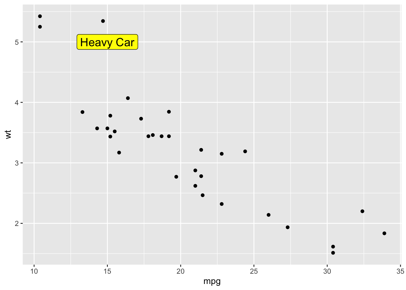
2️) Adding a Label with a Background
mtcars |>ggplot() +aes(x = mpg, y = wt) +geom_point() +annotate(geom ="label", x =15, y =5, label ="Heavy Car", fill ="yellow", color ="black", size =5)