Based Plot: Histogram
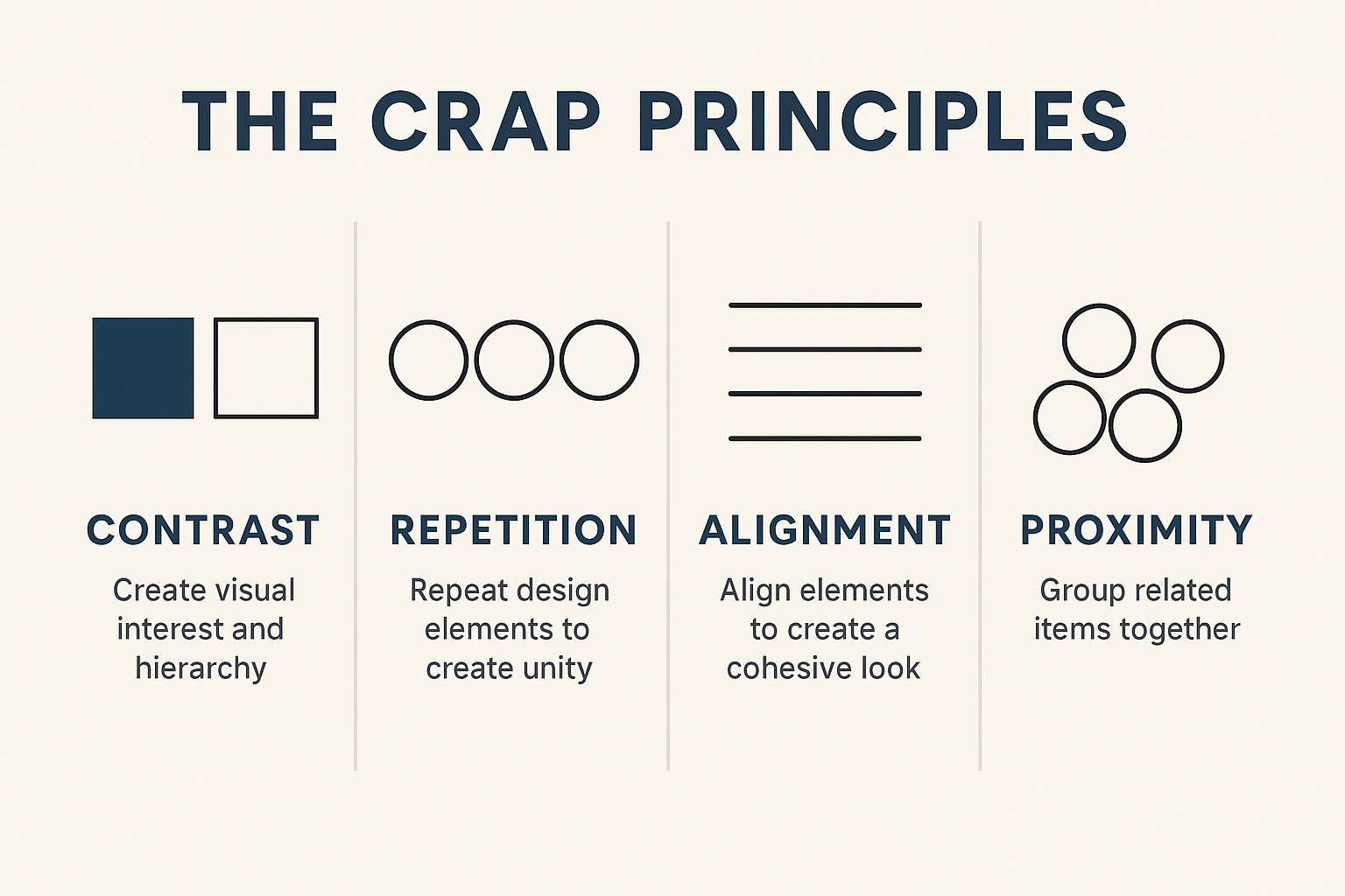
The CRAP principles are a set of design guidelines that help make layouts more organized, visually appealing, and easy to understand. CRAP stands for:
Contrast: Create visual contrast between elements, like varying sizes, colors, and font styles. This helps highlight important information and makes it easier for viewers to distinguish different sections.
- Example: Use bold, bright colors for headings and lighter shades for body text.
Repetition: Repeat certain design elements, such as fonts, colors, or shapes, throughout the layout to create unity and consistency.
- Example: Use the same font and color scheme across all pages of a website.
Alignment: Arrange elements in a structured way to create a clean and organized appearance. Proper alignment helps the viewer’s eyes flow naturally across the page.
- Example: Align all text to the left, right, or center to maintain consistency rather than mixing alignments.
Proximity: Group related items together to show their connection and make the information easier to scan.
- Example: Place similar buttons (like “Submit” and “Cancel”) close to each other.
Using these CRAP principles can greatly enhance the readability, clarity, and visual appeal of designs for websites, posters, or any printed materials.
📊 Summary of R Commands Used (Histograms & Density Plots)
1. hist(): Creates a histogram (frequency distribution).
2. lines()
Adds lines to an existing plot.
Often used with
density()to add a smoothed curve.
Key arguments:
col→ line colorlwd→ line widthlty→ line type (solid, dashed, dotted, etc.)
3. density()
Estimates the probability density function of a numeric variable.
Returns an object that can be plotted with
plot()orlines().
4. plot(): General plotting function. Used here for density plots.
5. legend(): Adds a legend to a plot.
6. box()
Adds a box around the plot area (optional).
colcan set the box border color.
7. rug()
- Adds tick marks at actual data values along the x-axis.
- Useful in combination with density plots.
8. rgb()
Defines colors with transparency.
rgb(red, green, blue, alpha)where values range 0–1.Example:
rgb(1, 0, 0, 0.5)= semi-transparent red.
10. rnorm(): Generates random numbers from a normal distribution.
11. Advanced hist() with plot = FALSE
hist(..., plot = FALSE)→ stores histogram object without drawing.Access
h$mids(bin midpoints) andh$counts(bin frequencies) for custom coloring.